TTM4110: Pålitelighet og ytelse med simulering
The purpose of this course is to give an introduction to the conceptual and theoretical fundamentals of dependability and performance of ICT systems. Mathematical and software tools that can be used to analyse and dimension systems and network solutions are presented and basic issues are discussed.
# Chapter 1
## Functional and non-functional properties
Technical systems are described using two types of characteristics:
__Functional properties:__ Which functions are performed.
__Non-functional properties:__ How well these functions are performed.
These terms can be used to describe systems, let's say a car: The primary function of a car is to transport people and goods from one place to another. Non-functional properties include the carrying capacity, the maximum speed, whether the car starts when needed, whether it transports people and goods to destination without breaking down or causing accidents. These are the _performance_ (carrying capacity, speed) and _dependability_ (the car starts and fulfills its function) properties of the system. Along with the price they are rational arguments for comparing different designs.
When designing an ICT-system, the focus is mainly on the functions the system shall provide and how to implement them. However, in a real system, it is also crucial to concider non-functional properties such as dependability and performance. The non-functional requirements will have an impact on both the design and the cost of the system and determine its usability.
## Models
Every dependability and performance evaluation of a system, either based on mathemactical analysis, simulation or measurements, always relies on a _model_ of the system.
__Model:__ A model is an abstraction of the real or projected system.
There is no standard recipe to elaborate a good model of a system and trade-offs must be made. On one hand a model must include sufficient details to represent the system, but on the other hand less important details must be left out to enable simulation in a reasonable time. Assumptions must be made so that the model can be expressed analytically, but at the same time one must ensure that the model still describes the real world. The results derived from a model should be valid for the real system, not just for the model.
The description of the system itself and the identification of what to include in the model are essential, but not sufficient. How the environments influence the system and vice versa must also be concidered.
## Systems
A _system_ can be defined as a _regularly interacting_ or _interdependent group of items forming a unified whole_, where an item may be a sytem, a subsystem, or an atomic component. When performing a dependability and/or performance evaluation of a system, the aim is to identify the items (system components) that limit the dependability and/or performance. The _structure_ of the system reflects how these components interact. The interactions themselves are referred to as the _behavior_ of the system.
### System components
An ICT-system is composed of _system components_ of different types, for instance: processors (with processing capacity), hard disks (with storage capacity), transmission channels (with transmission capacity) and so on. These system components and their capacities are the _resources_ in an ICT-system. The amount of resources limits the system dependability and performance. The resources are what is utilized when the system is used.
### Structure
The _structure_ of a system indicates how the resources in the system must or should be utilized in order to deliver the service of which the dependability and/or performance properties are evaluated. The structure of a system may be physical, logical, or derived from the physical and/or logical structures.
### Behaviour
It is necessary to simplify and make an abstraction of the behavior of the real system. Important aspects of the behavior that may be included in a model may be:
1. _Queueing diciplines_: What to do when all resources in the system is busy and someone/something new wants to use the sysem.
2. _Protocols_: Provides rules for the different entities in a system/network so they can cooperate
3. _Traffic mechanisms_ apart from protocols: Routing algorithms, CAC, UPC and so on.
4. _Fault-handling_: Mechanisms which encompass error detection, localization, isolation, and various techniques to provide _fault tolerance_ and automatic and manual _fault removal_ (repair). Important to include the possibility that the system does not behave as intended, e.g. that an error in the system is not detected.
## Concepts and terminology
This section introduces concepts and terminology related to dependability and performance.
### Quality of service
__Quality of service (QoS)__: Degree of compliance of a service to the agreement that exists between the user and the provider of this service.
In this context, a _user_ is an entity that uses a service provided by another entity, but is not necessarily an end-user of the service. A _service_ is a set of functions (_service primities_) that are offered on an interface between the user and the provider (not necessarily a physical interface). A _QoS parameter_ is a (random) variable that characterizes the service.
### Dependability
__Dependability__: Trustworthiness of a system such that reliance can justifiable be placedo nthe service it delivers.
Dependability is a high-level concept. In addition to the _dependability attributes_ which will be discussed later, depndability also encompasses the _impairments_ that could affect the trustworthiness of a system, and the _means_ to attain dependability.
__Failure__: Deviation of the delivered service from the compliance with the specification. Transition from correct service to incorrect service (e.g. the service becomes unavailable.
__Error__: Part of the system state which is liable to lead to a failure.
__Fault__: Adjudged or hypothesized cause of an error.
Example: An electromagnetic pulse (fault) results in flipping of a bit in a data register (error). When this register is accessed, a wrong result is returned to the user (failure). Another example is the software engineer who writes an incorrect code and thereby introduces a logical fault into a software module. This incorrect code is a (dormant) fault embedded in the system. Certain input values will activate the fault and there will be an error in the service. Services delivered by the software module may later crash or produce incorrect output (failure).
Two basic approaches to achieve a dependable system:
_fault prevention_, i.e. to prevent the occurrance or introduction of faults.
_fault tolerance_, i.e. to prevent that errors cause failures, or in other words, to deliver a correct service despite the presense of faults.
Types of faults: Physical faults (physical wear on components), transient faults (only present for a short period of time), intermittent faults (faults come and go), design faults (Human made faults during specification, design and implementation of a system), interaction or operational faults (Accidental faults made by humans operating or maintaining a system), and environmental faults (faults originating outside the system bounderies).
__Availability__: Ability of a system to provide a set of services at a given instant of time or at any instant within a given time interval.
__Reliability__: Ability of a system to provide uninterrupted service.
__Safety__: Ability of a system to provide service without the occurance of catastrophic failures.
### Performance
__Performance__: Ability of a system to provide the resources needed to deliver its services.
__Capacity__: Maximum load a system can handle per time unit.
## Use of modeling in development and dimensioning.
TODO
## Random extensions
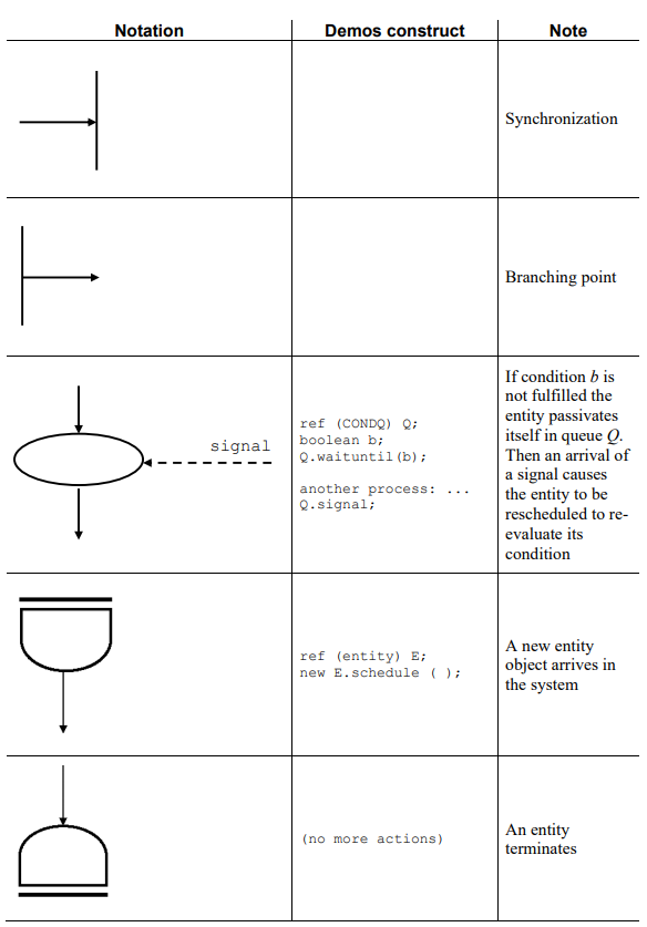
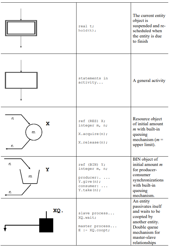
### Activity diagram
__Point process__
- Point process describes occurrence of an event
- No gradation of type of event
- The state, X(t), of a process is the number of events, N(t)
_Regular point process_ only one event at a time.
> Time to k'th event:
$$ S_k = \sum_{i=1}^k Y_i $$
har også at
$$ P(N(t)<k) = P(S_k>t) $$
sd
__Renewal process__
Regular point processes
Time to next event is independent of what happened in the past
The superposition of merging two renewal processes is generally __not__ a renewal process.
However, the superposition of a large number of renewal processes tends to a Poisson process.
__Little's formula__:
$$ \overline{N} = λ\hat{W} $$
N is avarage for N(t).
W is avarage for all
__Erlang__: Erlang is a dimensionless unit that is used as a measure for offered load or carried load from service-providing elements.
Often expressed as call arrival rate times average call length.
Given a scenario with a single cord in telephone system. The cord can provide phone calls for 60 minutes per hour. A full utilization of the cord results in 1 erlang.
If users now attempts to make calls in this system (measured in eg. per hour):
* Carried load is the traffic that was carried for the successful call-attempts.
* Offered load is the traffic that would have been carried if all the call-attempts succeeded.
Offered traffic (in erlangs) is related to the call arrival rate, λ, and the average call-holding time (the average time of a phone call), h, by:
$$ E = λh $$
provided that h and λ are expressed using the same units of time (seconds and calls per second, or minutes and calls per minute).
__Relative frequency__:
Number of times the event occurs divided by the number of
times an experiment is carried out
__Probability__:
Asymptotic relative frequency of the event investigated
__Joint probability__:
The probability that both events occurs in conjunction
(Intersection) $ P(A ∩ B) $
__Conditional probability__:
If A and B are two events, and P(B) > 0
P(A|B) = P(A ∩ B)
P(B)
Multiplicative rule
P(A ∩ B) = P(A|B)P(B)
Law of total probability:
P(B) = P
j P(B ∩ Aj) = P
j P(B|Aj) · P(Aj)
__Negative exponential distribution__:
X ∼ Exp(λ)
$$ f(x) = λe^{−λx}, x ∈ R^+ $$
$$ F(x) = 1 − e^{−λx} $$
where $λ ∈ R^+$ is the rate parameter
__Erlang-k distribution__: It is the distribution of the sum of k random variables identically distributed.
X ~ Erlang-k(λ)
$$ f(x) = \frac{(λx)^{k−1}}{(k − 1)!} λe^{−λx}$$
Der $x ∈ R^+$
__Binomial distribution__:
Probability distribution of the number X of events 1 in a
sequence of n independent Bernoulli trials.
X ∼ Bin(n, p)
$$f(x) = \binom{n}{x} p^x (1-p)^{n-x} $$
Der $x ∈ $ {0, 1, ...}
__Poisson distribution__:
Corresponds to the binomial distribution with an infinite number
of Bernoulli trials.
Probability of the number of occurrences of an event, given
that it occurs on average at the intensity $α ∈ R^+$
X ∼ P(α)
$$ f(x) = \frac{α^x}{x!} e^{-α} $$
$x ∈ N$
__Poissoon process__:
> TODO: format
• Regular point process (only one event at the time)
• Intensity is constant (homogeneous PP)
• Intensity is independent of previous events
The merging (superposition, multiplexing) of two Poisson
processes is a Poisson process
Splitting of a Poisson process in n processes forms n
Poisson processes if the splitting is probabilistic (with
constant probability)
## Queueing model
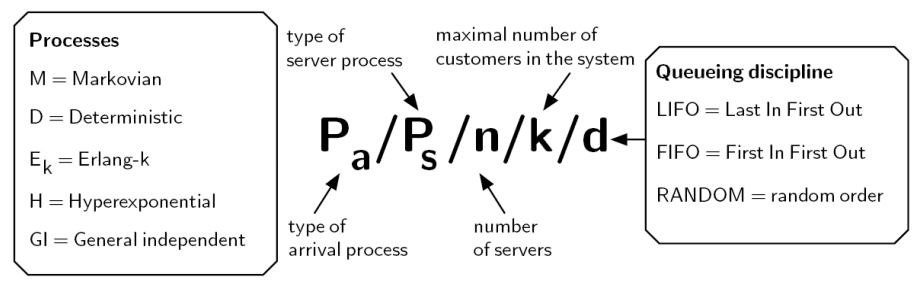
### Kendall's notations:
> TODO: format
__Examples__
Kendall’s notation, example: M/M/1
– M = Poisson arrival process
– M = service time distribution is n.e.d.
– 1 server
– No system capacity given, i.e. infinite
– No queuing discipline, i.e. arbitrary discipline can be
used
• Infinite server systems: M/M/∞
• Loss systems: M/M/n/n
• Delay systems with infinite queue: M/M/n
• Jackson’s queueing network: network of M/M/nj -system
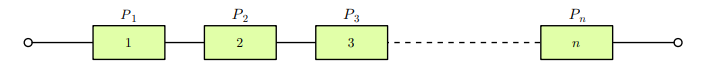
### Series system:
__Expected value__: $ µ = E(X) $
__Variance__: $ σ^2 = Var(X) = E[(X-µ)^2] = E(X^2) - µ^2 $
__Standard deviation__: $ σ = \sqrt{Var(X)} $