System : A system can be defined as a regularly interacting or interdependent group of items forming a unified whole. Every dependability and performance evalutation of a system, either based on mathmatical analysis, simulation or measurements, always relies on a model of the system. Model : A model is an abstraction # Functional and non-functional properties Technical systems are described using two types of characteristics: Functional properties : Which functions are performed. Non-functional properties : How well the functions are performed. For example: carrying capacity, speed, whether the system performs its function, delay, safety, blocking probability. # The System A system can be defined as a regularity or interdependent # Faults Physical faults : Physical faults, or solid faults, are the "classical"faults, e.g wear out of components, random device defects due to manufacturing imperfections, physical degradation of the material of the component as a result of electrical overstress, pollution, mechanical stress or shock. Physical faults are internal to the system. They are permanent, that is, as soon as the physical fault has occured it persists until reparied. They occur in the operational phase of the life cycle of system, both during use and inactivity (in store, serving as a back up or simply powered off). 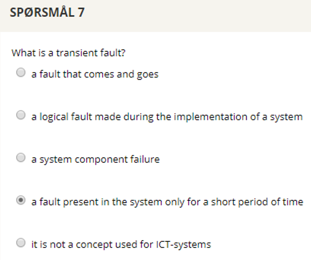Transient faults : Transient faults are present only for a short period of time and no physical change occurs in the system. Transient faults are usually caused by disturbances external to the system itself like electromagnetic interference and radiation. Typical transient fautls are noise on a transmission line and alpha-particles passing through RAM flipping bits. Transient fautls occur during the operational phase of the life cycle of a system and have a physical origin. In practise, it may be very difficult to distinguish between transient and intermittent faults Intermittent faults : Intermittent faults, or sporadic faults, come and go. They may be due to changes of the parameters of a hardware component caused by tempoerature, aging etc., marginal timing, synchronization in hardware or software, specific input patters, etc. Intermittent faults may have a physical or human origin. They are problematic to deal with since they are very difficult to localize and correct. Many dependability predictions take only permanent physical faults into consideration. There are several investigations showing that temporary physical fualts (transient and intermittent) are far more frequent. # Models Every dependability and performance evaluation of a system, either based on mathemactical analysis, simulation or measurements, always relies on a _model_ of the system. __Model:__ A model is an abstraction of the real or projected system. There is no standard recipe to elaborate a good model of a system and trade-offs must be made. On one hand a model must include sufficient details to represent the system, but on the other hand less important details must be left out to enable simulation in a reasonable time. Assumptions must be made so that the model can be expressed analytically, but at the same time one must ensure that the model still describes the real world. The results derived from a model should be valid for the real system, not just for the model. The description of the system itself and the identification of what to include in the model are essential, but not sufficient. How the environments influence the system and vice versa must also be concidered. ## Systems A _system_ can be defined as a _regularly interacting_ or _interdependent group of items forming a unified whole_, where an item may be a sytem, a subsystem, or an atomic component. When performing a dependability and/or performance evaluation of a system, the aim is to identify the items (system components) that limit the dependability and/or performance. The _structure_ of the system reflects how these components interact. The interactions themselves are referred to as the _behavior_ of the system. ### System components An ICT-system is composed of _system components_ of different types, for instance: processors (with processing capacity), hard disks (with storage capacity), transmission channels (with transmission capacity) and so on. These system components and their capacities are the _resources_ in an ICT-system. The amount of resources limits the system dependability and performance. The resources are what is utilized when the system is used. ### Structure The _structure_ of a system indicates how the resources in the system must or should be utilized in order to deliver the service of which the dependability and/or performance properties are evaluated. The structure of a system may be physical, logical, or derived from the physical and/or logical structures. ### Behaviour It is necessary to simplify and make an abstraction of the behavior of the real system. Important aspects of the behavior that may be included in a model may be: 1. _Queueing diciplines_: What to do when all resources in the system is busy and someone/something new wants to use the sysem. 2. _Protocols_: Provides rules for the different entities in a system/network so they can cooperate 3. _Traffic mechanisms_ apart from protocols: Routing algorithms, CAC, UPC and so on. 4. _Fault-handling_: Mechanisms which encompass error detection, localization, isolation, and various techniques to provide _fault tolerance_ and automatic and manual _fault removal_ (repair). Important to include the possibility that the system does not behave as intended, e.g. that an error in the system is not detected. ## Concepts and terminology This section introduces concepts and terminology related to dependability and performance. ### Quality of service __Quality of service (QoS)__: Degree of compliance of a service to the agreement that exists between the user and the provider of this service. In this context, a _user_ is an entity that uses a service provided by another entity, but is not necessarily an end-user of the service. A _service_ is a set of functions (_service primities_) that are offered on an interface between the user and the provider (not necessarily a physical interface). A _QoS parameter_ is a (random) variable that characterizes the service. 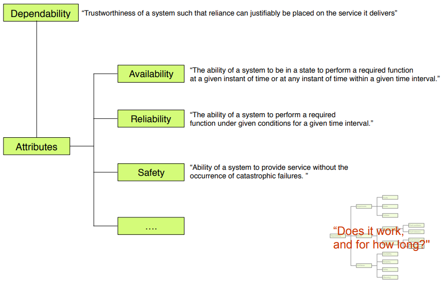### Dependability __Dependability__: Trustworthiness of a system such that reliance can justifiably be placed on the service it delivers. __Failure__: Deviation of the delivered service from the compliance with the specification. Transition from correct service to incorrect service (e.g. the service becomes unavailable. __Error__: Part of the system state which is liable to lead to a failure. 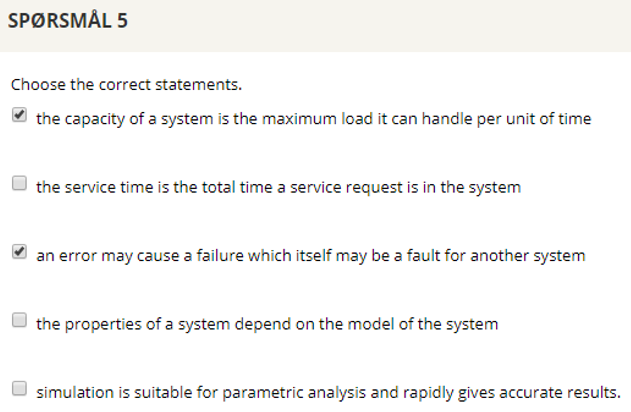__Fault__: Adjudged or hypothesized cause of an error. Example: An electromagnetic pulse (fault) results in flipping of a bit in a data register (error). When this register is accessed, a wrong result is returned to the user (failure). Another example is the software engineer who writes an incorrect code and thereby introduces a logical fault into a software module. This incorrect code is a (dormant) fault embedded in the system. Certain input values will activate the fault and there will be an error in the service. Services delivered by the software module may later crash or produce incorrect output (failure). Two basic approaches to achieve a dependable system: _fault prevention_, i.e. to prevent the occurrance or introduction of faults. _fault tolerance_, i.e. to prevent that errors cause failures, or in other words, to deliver a correct service despite the presence of faults. Types of faults: Physical faults (physical wear on components), transient faults (only present for a short period of time), intermittent faults (faults come and go), design faults (Human made faults during specification, design and implementation of a system), interaction or operational faults (Accidental faults made by humans operating or maintaining a system), and environmental faults (faults originating outside the system bounderies). __Availability__: Ability of a system to provide a set of services at a given instant of time or at any instant within a given time interval. __Reliability__: Ability of a system to provide uninterrupted service. __Safety__: Ability of a system to provide service without the occurrence of catastrophic failures. ### Performance __Performance__: Ability of a system to provide the resources needed to deliver its services. __Capacity__: Maximum load a system can handle per time unit. __Throughput__: Portion of the system capacity that is utilized by the users. __Delay__: Time it takes to complete a service. 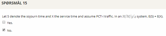__Waiting time__: Accumulated time a service reuqest is pendingfor service in a system.(W) __Service time__: Accumulaed time a service request is served by a system. (X) __Sojourn time__: Total time a service request is in a system. (S = W + X) ## Methods: ### Mathematical analysis In the case of a well-known probelm, results are rapidly and easily obtained using formulas or algrotihms. Explicit parametric relations can be found for simple models, and parametric analysis, e.g. sensitivity analysis, is relatively easy. ### Simulation: Relatively detailed and realistic models can be used. Simulation allows o use system models with an arbitrary level of deatils. The challenge is to include all that is relevant for the evaluation but nothing more. A lower level of knowledge is required to design new models ### Measurement on prototype of a system Results are trustworthy since they are not affected by assumptions and simplifications. Results are realitic and detailed. # Chapter 2: Fundamentals of probability Not completed yet, feel free to contribute here.  __Expected value__: $ µ = E(X) $ __Sample mean (avarage)__: $ µ \approx \overline{X} = \frac{1}{n} \sum_{i=1}^n X_i $ __Variance__: $ σ^2 = Var(X) = E[(X-µ)^2] = E(X^2) - µ^2 $ __Sample variance__: $ S^2 = \frac{1}{n-1} \sum_{i=1}^n (x_i-\overline{x})^2 $ $ S^2 = \frac{1}{n-1} \sum_{i=1}^n (x_i^2 - 2\overline{x}x_i + \overline{x}^2)^2 $ $ S^2 = \frac{1}{n-1} \sum_{i=1}^n x_i^2 - 2\overline{x}\sum_{i=1}^nx_i + n\overline{x}^2 $ $ S^2 = \frac{1}{n-1} \sum_{i=1}^n x_i^2 - n\overline{x}^2 $ __Standard deviation__: $ σ = \sqrt{Var(X)} $ __Standard error__: $ SE = \sqrt\frac{σ^2}{n} = \frac{σ}{\sqrt n} ≈ \frac{S}{\sqrt n} $ __Intensity__: $ E(X) = \frac{1}{γ} \rightarrow E(\hat{X}) = \hat{γ} $ __Conditional probability__: $ P(A | B) = \frac{P(A ∩ B)}{P(B)} $ __Baye's formula__: $ P(A | B) = \frac{P(B | A) · P(A)}{P(B)} $ __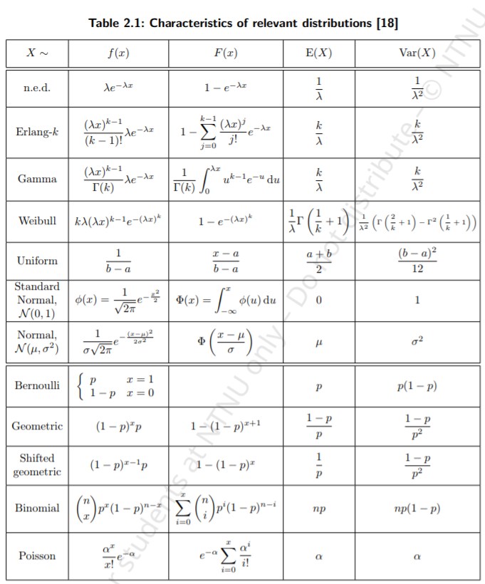Negative exponential distribution (n.e.d) (probability density function)__: $ f(x) = λe^{−λx} $ or cumulative: $ F(x) = 1 − e^{−λx} $ __Erlang -k distribution probability density function (k is shape and λ is rate of each phase)__: $ f(x) = \frac{(λx)^{k−1}}{(k − 1)!} λe^{−λx} $ and cumulative: $ F(x) = 1 − e^{−λx} \sum_ {j=0}^{k-i} \frac{(λx)^j}{j!} $ __Death rate (failure rate)__: $ φ(t) = \frac{f(t)}{1 − F(t)} $ # Chapter 4: Simulation ## Simulation Imitative representaion of the functioning of one system or process by means of the functioning of another. In the context of this course: A simulation is performed by means of a software program, called a simulator, running on a computer. By simulation, we really mean stochastic simulation where the behaviour of the system components is, fully or partly, governed by stochastic processes. To imitate a stochastic behavior, the simulator, and therefore the computer, has to be able to generate random variables according to a given probability distribution. ### Random variable generation: Simulation reilies on the generation of random variables, and therefore on the generation of random numbers. Generated random variables are called _random variates_. Random numbers may be generated either from a physical process or from an algorithm. The main drawback of generating random numbers from a physical process is that the sequence is not reproducible. Generating random numbers from an algorithm using a computer allows to generate a large amount of numbers and to reproduce the same sequence several times which enables to reproduce the same experiments. Random numbers generated by an algorithm are not truly random since the algorithm itself is deterministic and are therefore called _pseudo-random numbers_. However, the sequence of numbers generated should appear to be _statisically random_ (independent and uniformly distributed random numbers). Requirements: Fast (many samples), portable, long cycle period, reproducible sequences, good statistical properties. #### Direct method: __Pro__: Fast, empirical distribution __Con__: Only applicable to discrete distributions. #### Inverse Transform: __Pro__: Fast __Con__: Distributions require a closed form inverse transform. #### Acceptance-Rejection: __Pro__: Many distributions. __Con__: Many samples per random variate generated. #### Convolution: __Pro__: Simple implementation of complicated distributions. __Con__: Only applicable to sum of variates. ## Advantages and disadvantages of simulation Simulation is a flexible and practical way of analyzing systems. Simulation allows to make models that include exactly the necessary level of granularity, not more not less. A simulation model is better tailored for a given study than a mathematical model or a real system. A mathematical model often needs to be prohibitevely simplified to be solved analytically. A real system used for a measurement study can obviously not be simplified at all. A simulation model is often more challenging and more demanding with respect to the insight into the system and the understanding of its operation. One must be able to remove unnecessary details and at the same time understand and describe the details of importance for a given study. Hence, a common and important by-product of a simulation study is an improved insight into the system and the identification of possible weaknesses in the design. ## Types of simulation models Simulation can be classified as static or dynamic, discrete or continuous, and deterministic or stochastic. In this course we use dynamic, discrete, and stochastic simulation models. ### Static simulation model Also called Monte-Carlo simulation models a particular point in time (time not part of model) E.g throwing a dice. ### Dynamic simulation model Model represents a system as it changes over time. E.g. simulate a bank from 08:00-16:00. ### Discrete simulation model State variables change only at discrete set of points in time. ### Continuous simulation model State variable changes continuously over time. ### Deterministic simulation model Contains no random variables. ### Stochastic simulation model Contains at least one random input variable ## Discrete event simulation (DES): The system dynamics is given by discrete events. The system state is distinct and will only change at a specific time instance. Simulations of discrete events need only to simulate the events that change the system state, and a finite number of events will take place in a finite interval of time. ## Time driven vs. event-driven simulation: Time driven: Fixed time stamp. For example: Move the clock 1 second forward and determine the system state. Event driven: Variable time-stamp. For example: Move the clock to the time of next event. ## Concepts in Discrete event simulation: __Model__: Abstract representation of system. __Entity__: Object with explicit model description. __Attributes__: Properties of an entity. __System__: Collection of entities. __System state__: Set of variables containing sufficient information. __List__: Collection of associated entities. __Event__: Change of system state. __Event notice__: A record of an event to occur. __Event list__: List of event notices (ordered by time) __Activity__: Specified duration. __Delay__: Unspecified duration. __Resource__: Passive object used to perform an activity. ## Process oriented simulation: A Process describes the behaviour of an entity (sequence of activities, life cycle). Focus on the entities and their dependencies and interactions (object-oriented approach). Event-driven approach. Requires a list of events and synchronization mechanisms. 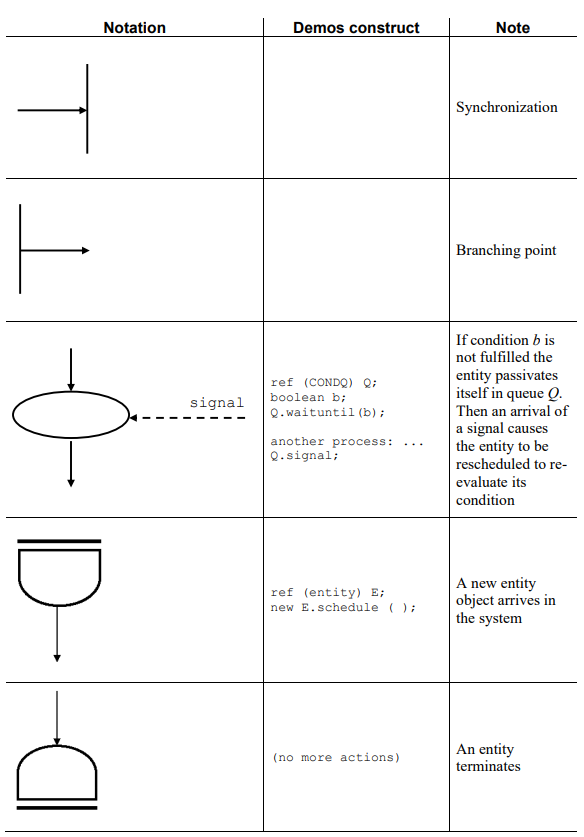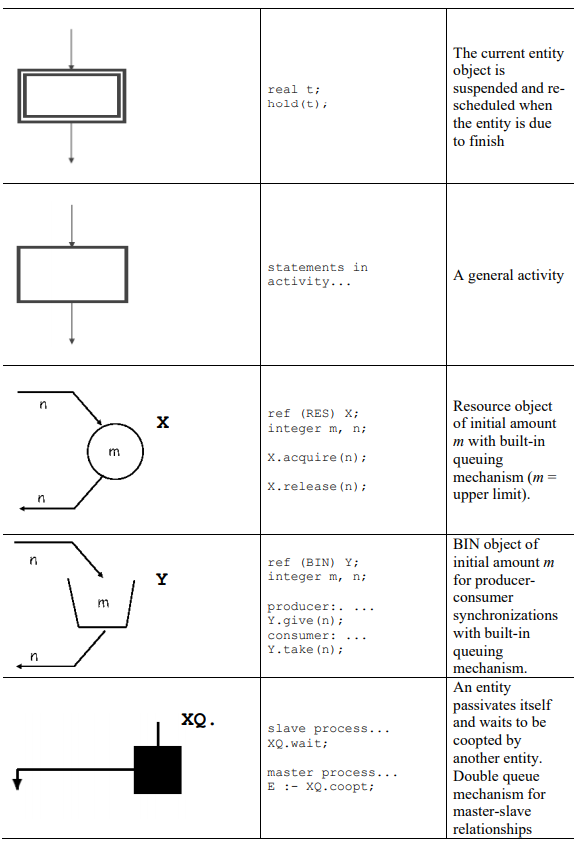## Activity diagram: A graphical representation of a model. Activites/life-cycles of entities. Interactions between entities (cooperation, interrupt, generation, priorities). Entities and resources (comptetition, synchronization).   # Chapter 5: Traffic Models This chapter presents the Poisson process and its properties. In particular, it describes how Poisson processes can be aggregated to form Markov processes that are an important part of Markov models. ## Poisson and Markov Process __Poisson process__: Regular point process (only one event at the time). Intensity is constant (homogenous PP). Intensity is independent of previous events. __Markov process__: Events from many Poisson Processes. __Poisson distribution__: Number of events until and including time t. __Exponential distribution__: Time between two consecutive events. ### Poisson process -merging The merging (superposition, multiplexing) of two Poisson processes is a Poisson process. Splitting of a Posson process in n processes forms n Poisson processes if the splitting is probabilitstic (with constant probability). ## Stationary traffic models ### Examples of queuing systems Phone subscirbers share a limited number of telephone lines in a telephone exchange Mobile phone subscribers share a limited number of radio transmitters/receivers in a mobile base station. Taxi call centers have delay queues. IP routers have input and output buffers. Maintenance centers have order lists and repairmen. __Performance__: Delay, blocking, utilization, waiting time... ### Queuing model A system does not need to have any queuing positions to be classified as a __queuing system__. A queueing system is characterized by the arrival process, service time distribution, number of servers, maimum number of customers in the system, number of sources, and queuing dicipline (service order). # Random extensions ## Use of modeling in development and dimensioning. 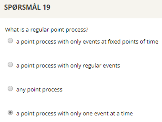TODO __Point process__ - Point process describes occurrence of an event - No gradation of type of event - The state, X(t), of a process is the number of events, N(t) _Regular point process_ only one event at a time. 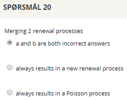> Time to k'th event: $$ S_k = \sum_{i=1}^k Y_i $$ har også at $$ P(N(t)<k) = P(S_k>t) $$ sd __Renewal process__ Regular point processes Time to next event is independent of what happened in the past The superposition of merging two renewal processes is generally __not__ a renewal process. However, the superposition of a large number of renewal processes tends to a Poisson process. __Little's formula__: $$ \overline{N} = λ\hat{W} $$ N is avarage for N(t). 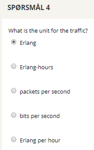W is avarage for all __Erlang__: Erlang is a dimensionless unit that is used as a measure for offered load or carried load from service-providing elements. Often expressed as call arrival rate times average call length. Given a scenario with a single cord in telephone system. The cord can provide phone calls for 60 minutes per hour. A full utilization of the cord results in 1 erlang. If users now attempts to make calls in this system (measured in eg. 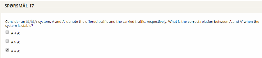per hour): * Carried load is the traffic that was carried for the successful call-attempts. * Offered load is the traffic that would have been carried if all the call-attempts succeeded. Offered traffic (in erlangs) is related to the call arrival rate, λ, and the average call-holding time (the average time of a phone call), h, by: $$ E = λh $$ provided that h and λ are expressed using the same units of time (seconds and calls per second, or minutes and calls per minute). __Relative frequency__: Number of times the event occurs divided by the number of times an experiment is carried out __Probability__: Asymptotic relative frequency of the event investigated __Joint probability__: The probability that both events occurs in conjunction (Intersection) $ P(A ∩ B) $ __Conditional probability__: If A and B are two events, and P(B) > 0 P(A|B) = P(A ∩ B) P(B) Multiplicative rule P(A ∩ B) = P(A|B)P(B) Law of total probability: P(B) = P j P(B ∩ Aj) = P j P(B|Aj) · P(Aj) __Negative exponential distribution__: X ∼ Exp(λ) $$ f(x) = λe^{−λx}, x ∈ R^+ $$ $$ F(x) = 1 − e^{−λx} $$ where $λ ∈ R^+$ is the rate parameter __Erlang-k distribution__: It is the distribution of the sum of k random variables identically distributed. X ~ Erlang-k(λ) $$ f(x) = \frac{(λx)^{k−1}}{(k − 1)!} λe^{−λx}$$ Der $x ∈ R^+$ __Binomial distribution__: Probability distribution of the number X of events 1 in a sequence of n independent Bernoulli trials. X ∼ Bin(n, p) $$f(x) = \binom{n}{x} p^x (1-p)^{n-x} $$ Der $x ∈ $ {0, 1, ...} __Poisson distribution__: Corresponds to the binomial distribution with an infinite number of Bernoulli trials. Probability of the number of occurrences of an event, given that it occurs on average at the intensity $α ∈ R^+$ X ∼ P(α) $$ f(x) = \frac{α^x}{x!} e^{-α} $$ $x ∈ N$ __Poissoon process__: > TODO: format • Regular point process (only one event at the time) • Intensity is constant (homogeneous PP) • Intensity is independent of previous events The merging (superposition, multiplexing) of two Poisson processes is a Poisson process Splitting of a Poisson process in n processes forms n Poisson processes if the splitting is probabilistic (with constant probability) ## Queueing model ### Kendall's notations: > TODO: format  __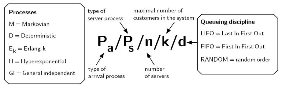Examples__ 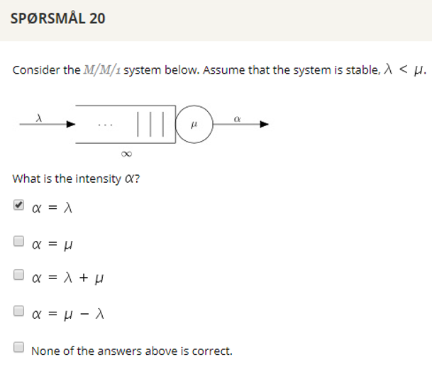Kendall’s notation, example: M/M/1 – M = Poisson arrival process – M = service time distribution is n.e.d. – 1 server – No system capacity given, i.e. infinite – No queuing discipline, i.e. 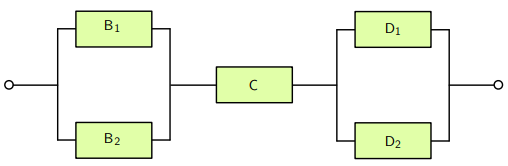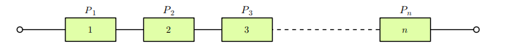arbitrary discipline can be used • Infinite server systems: M/M/∞ • Loss systems: M/M/n/n • Delay systems with infinite queue: M/M/n • Jackson’s queueing network: network of M/M/nj -system ## Dependability  ### Series system:  __Availability__: $$ A_{series} = \prod_{i=1}^n X_i $$ __Reliability function__: $$ R_{series}(t) = \prod_{i=1}^n R_i(t) $$ der $ R_i(t) = e^{-λ_it} $ ### Parallel system:  __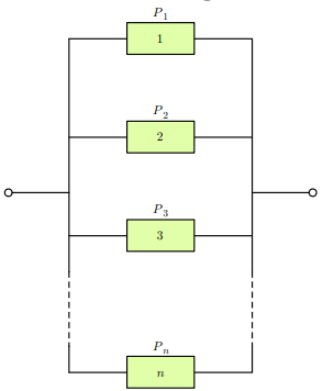Availability__: $$ A_{parallel} = 1 - \prod_{i=1}^n (1-X_i) $$ __Reliability function__: $$ R_{parallel}(t) =1 - \prod_{i=1}^n (1-R_i(t)) $$ ### K-of-n system:  __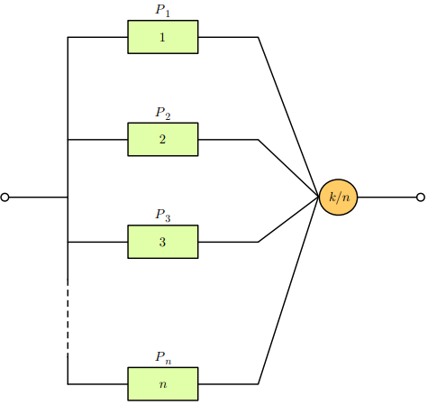Availability__: $$ A_{k-of-n} = \sum_{i=k}^n \binom{n}{i} A^i (1-A)^{n-i} $$ __Reliability function__: $$ R_{k-of-n}(t) = \sum_{i=k}^n \binom{n}{i} R(t)^i (1-R(t))^{n-i} $$ ### 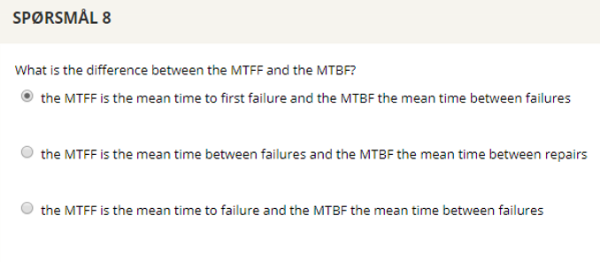Mean Time to First Failure: $$ MTFF = E(T_{FF}) = \int_0^∞ R(t)dt $$ ### Mean Time to Catastrophic Failure: $$ MTCF = E(T_{CF}) $$ ### Mean Time Between Failures: $$ MTBF = E(T_{BF}) $$ ### 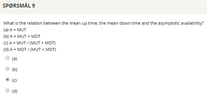Mean Up Time: $$ MUT = E(T_U) $$ ### Mean Down Time: $$ MDT = E(T_D) $$ ### Mean Time To Failure: $$ MTTF = E(T_F) = \int_0^∞ R(t) dt $$ ### Mean Time to First Failure: For a system that cannot be repaired and a structure of independent elements with constant failure rate $λ_i$ $(λ = λ_i, ∀i)$. 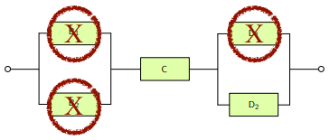$$ MTFF_{series} = (\sum_{i=1}^n λ_i)^{-1} $$ $$ MTFF_{parallel} = \frac{1}{λ} \sum_{i=1}^n \frac{1}{i} $$ $$ MTFF_{k-of-n} = \frac{1}{λ} \sum_{j=k}^n \frac{1}{j} $$ ### How to improve system availability: - Identify the most critical factor (element) in the system model - Set element availability to 1 - Calculate the net change in system availability - Repeat for all elements - Which element has the larges impact on the system availability? - What does it take to improve that element? - Alternatives: - Replacement of a component with lower failure rate - Improve recovery time - Change the structure by adding more ## Cut set __Cut set__ > The system fails if all elements in the set fails __Minimum cut set__ > The system fails if and only if (iff) when all elements in the set fail, given that the system elements not in the set are working  ## Path set __Path set__ > The system is working if all elements in the set are working __Minimum path set__ > The system is working iff all elements in the set are working, given that all system elements not in the set are failed. 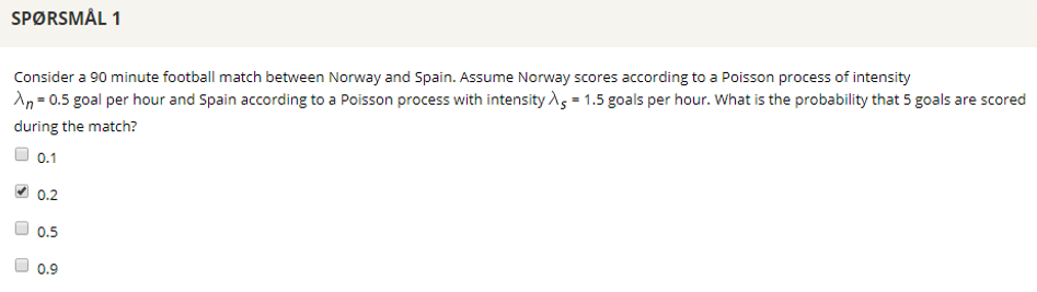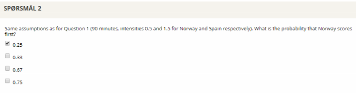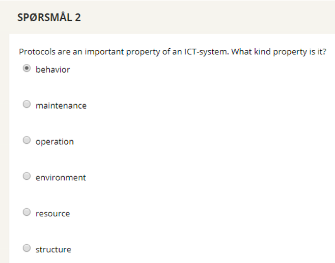### Example:  # Selftest 1: ## Question 1  ## Question 2  The main purpose of a protocol is to provide rules for the different entities in a system/network to cooperate. In other words a protocol dictates how various system parts interact with eachother, and is thus part of the __behaviour__ property of the system. 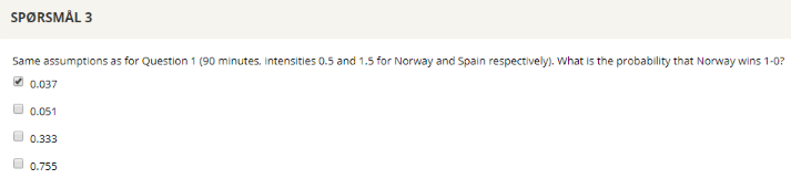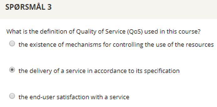## Question 3  Definition from the book: Quality of Service (QoS) is the degree of compliance of a service to the agreement that exists between teh user and the provider of this service. 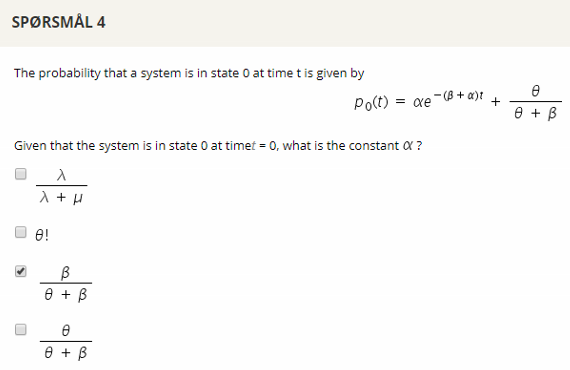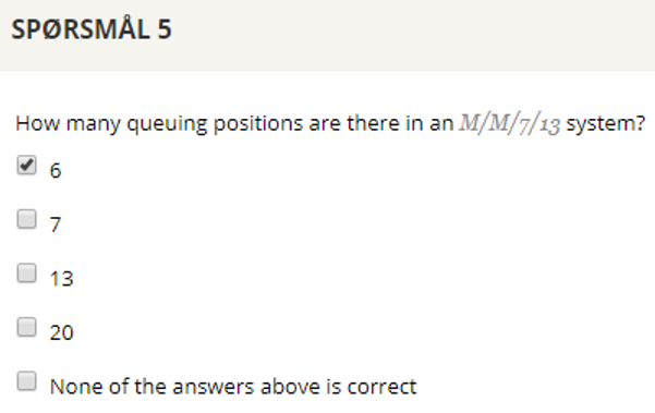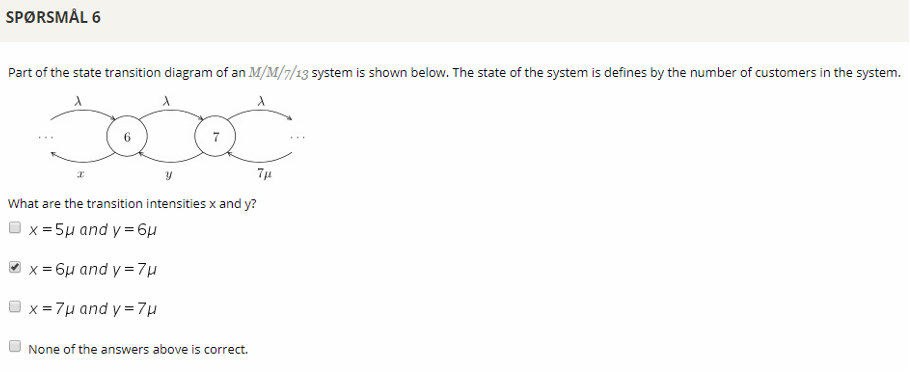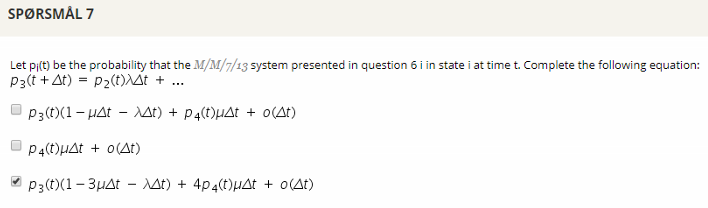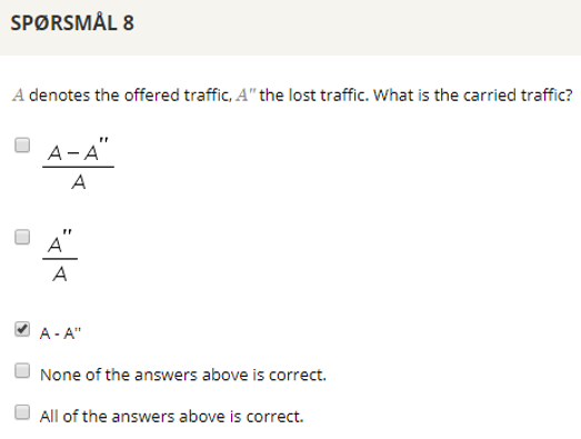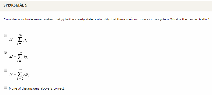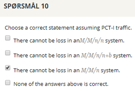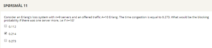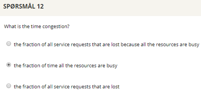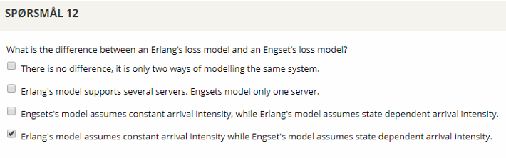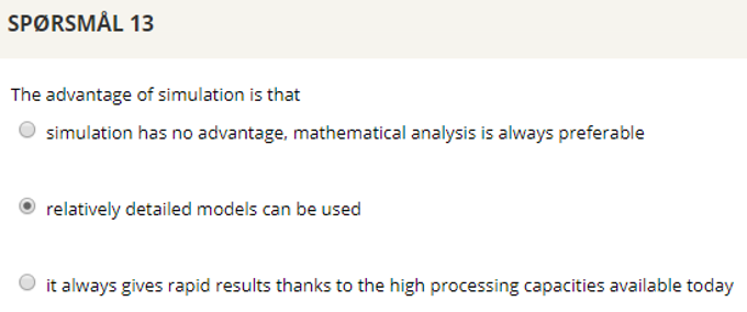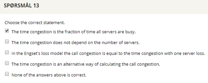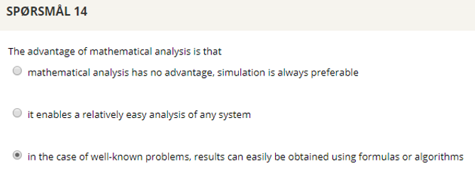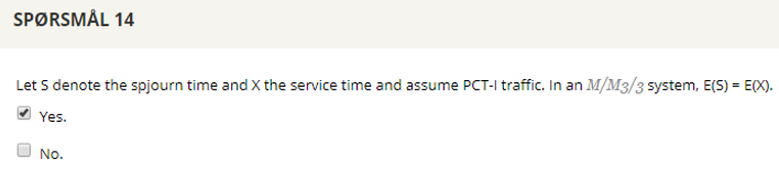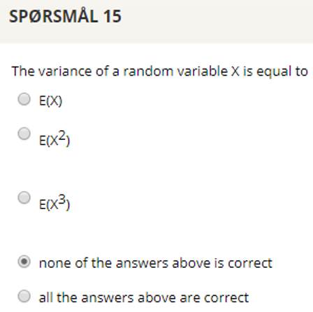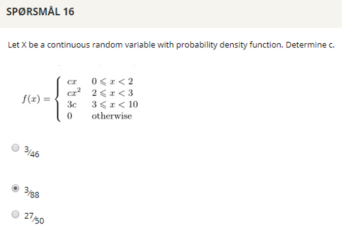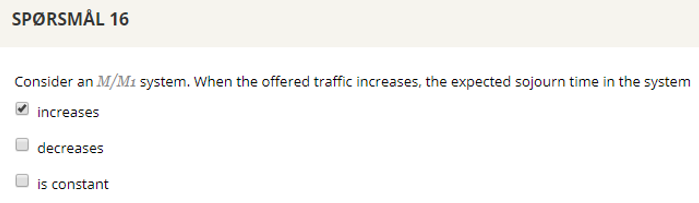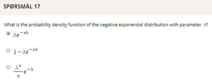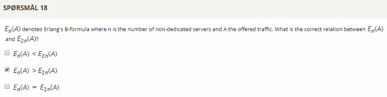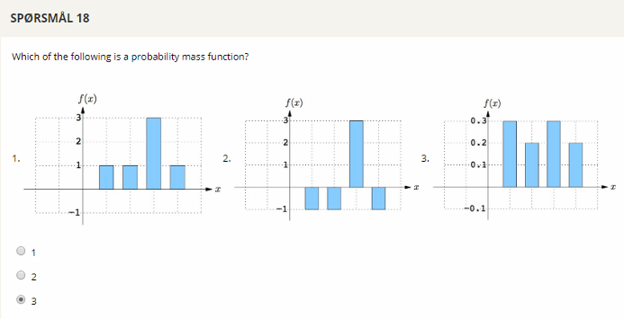## Question 4  ## Question 5  ## Question 6  ## Question 7  ## Question 8  ## Question 9  ## Question 10  ## Question 11  ## Question 12  ## Question 13  ## Question 14  ## Question 15  ## Question 16  ## Question 17  ## Question 18  Individual probabilities must be between 0 and 1. The sum of all probabilities must equal 1. 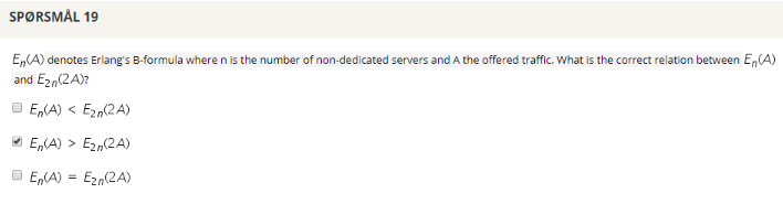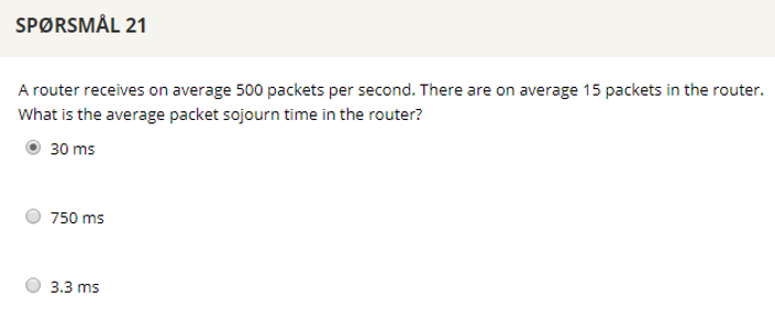## Question 19  ## Question 20  ## Question 21  15/500 = 0.03 # Selftest 2 ## Question 1  ## Question 2  ## Question 3  ## Question 4  ## Question 5  ## Question 6  ## Question 7  ## Question 8  ## Question 9  ## Question 10  ## Question 11  ## Question 12  ## Question 13  ## Question 14  ## Question 15  ## Question 16  ## Question 17  ## Question 18  ## Question 19  ## Question 20