TTT4135: Multimedia Signal Processing
This is work in progress. Will be completed while reading to the exam
Part 1: Statistical characterization of audiovisiual information
1.1: Digitization
We want to digitize our signals for multiple reasons. Digital signals is more robust to noise introduced by storage and transmission. It allows for inclusion of error protection and makes encryption possible. It allows us to integrate speech and image so that the data is independent of the network. It makes packet transmission over the internet possible, and introduces the possibility of integration between transmission and switching. We can use digital signal processing on the digitized information, and it conforms with the development of moder digital circuits

1.1.1: Digital Speech
- Bandwidth: 50-3400 Hz
- Sampling: 8 KHz
- Representation: 8 bit Log PCM (13 bit linear PCM)
- Dynamic range: 42 dB
- Characterization:
- Spectral components
- Component description (phonemes)
Digital speech is often presented as a spectrum (frequency/Amplitude) or spectrogram (frequency/time/amplitude)
1.1.2: Digital images/video
- Many proprietary formats, .flv, .avi, .mp4 etc. *Rates go from ~20kbps to 27 Mbps
Images has significant correlation between spectral components. The colors doesnt really matter, and conversion between different color spaces can be done fairly easy. There is significant correlation between neighbouring pixels. This means that we really dont have to treat every pixel for itself, but can instead look on a larger area of pixels. Natural images often exhibit large semi-uniform areas. Images are also non-stationary.
We have different tools for analysis and coding/compression of digital images.
- Analysis:
- Fourier transform in two dimensions
- Subband decomposition
- Coding/compression:
- Block transforms (DCT)
- Filter banks/Subband decomposition
- Wavelets
- General filters
- Prediction/estimation
- Motion compensation
- Quantization
- Entropy coding
1.2: Compression
For a source coder, the output should be efficient (compression), minimum distortion (fidelity) and robuts (reconstruction)  In the above picture we see the tradeoffs when dealing with coding. Time delay, compression ratio and complexity will all affect the overall recieved signal quality. There are three fundamental steps in compression; signal decomposition, quantisation, and coding.
1.2.1: Signal decomposition
Removes redundancy. Correlation between consecutive samples -- Can be removed reversible (without loss of information). This step can also be known as the sampling step usually involfing an A/D convertion.
When dealing with audiovisual content there are two ways we can reduce the size of the files. Alot of the signal contains redundancy, for example big areas of uniformity in an image. This can be removed reversible, without loss of information. Some of the content also contains irrelevancy, for example frequencies above the human hearing range in audio content. This is an irreversible operation.
1.2.2: Signal quantisation
Removes irrelevancy. Non-perceivable information -- Can be removed irreversibly (with loss of information). The quantisation can be described by:
\begin{equation} Q(s)=D(E(s)) \end{equation}
1.2.3: Signal coding
Transmit a perceptually relevant and statistically non redundant signal over the channel to the receiver. Makes the compression efficient.
The source coder output should be:
- Efficient (compression)
- Minimal distortion (fidelity)
- Robust (reconstruction)
1.3: Manipulation
1.4: Communications
1.5: Filtering
Part 2: Standards
2.1: Audio Compression
2.2: Image Compression
Image compression can be done either lossless or lossy. Lossless means that we can compress the images, and then decompress them and get the same image. With lossy compression, the images are altered in a way that it is not possible to recover the original images. We are mostly interested in lossy compression in this course, so the lossless formats will only be presented briefly
A picture is usally divided into slices, then macroblocks, then 8x8 pixel blocks.
The spectral redundancy can be removed by doing a color transform, for example YUV or grayscale conversion. The spatial redundancy reduction can be achieved with transform coding/subband decomposition and quantization. The temporal redundancy can be reduced by using motion compenstaion/estimation, predictive coding and temporal filtering. Entropy coding is a "free" way to get content more compressed. This can be achieved by using huffman coding or arithmetic coding.
2.2.1: Lossless formats
2.2.1.1: Tiff
Stands for "Tagged Image File Format". Can handle color depths from 1-24 bit. Uses Lempel-Ziv-Welch lossless compression. TIFF is a flexible, adaptable file format for handling images and data within a single file by including the header tags (size, definition, image-data arrangement, applied image compression). Can be a container holding lossy and lossless compressed images.
2.2.1.2: BMP
Short for "Bitmap". Developed by windows. Stores two-dimensional digital images both monochrome and color, in various color depths, and optionally with data compression, alpha channels and color profiles.
2.2.1.3: GIF
Stands for "Graphics Interchange Format". Can only contain 256 colors. Commonly used for images on the web and sprites in software programs
2.2.1.4: PNG
Stands for "Portable Network Graphics". Supports 24-bit color. Supports alpha channel, so that an image can have 256 levels of transparency. This allows designers to fade an image to a transparent background rather than a specific color.
2.2.2: Lossy formats
2.2.2.1: JPEG
JPEG is waveform based, and uses DCT. The process of JPEG encoding is as follows; First we do a color transform to reduce spectral redundancy, from RGB to YCbCr. We segment into 8x8 blocks, and do a DCT of each block. For JPEG we have hard-coded quantization tables that quantizes the blocks. We do a zigzag coefficient scanning, and code with huffman or arithmetic coding followed by run-length coding
2.2.2.2: JPEG2000
JPEG2000 uses wavelets, and is used mainly for digital cinema. JPEG2000 is meant to complement, and not to replace JPEG. The most interesting additions is region of interest coding (ROI), better error resilience and more flexible progressive coding. It also allows lossy and lossless compression in one system. It provides better compression at low bit-rates. It is better at comput images and graphics, and better under error-prone conditions. It uses the discrete wavelet transform (DWT) instead of DCT for signal decomposition. This makes the artefacts from JPEG2000 "ringing", based on the removal of the high frequency components, instead of JPEGs blockiness.
Images may contain 1-16384 components, and sample pixel-values can be either signed or unsigned. It supports bit depth up to 38 bits. The first step is preprocessing of the images. The input images are partitioned into rectangular, non-overlapping tiles of equal size. The tile-size can vary from one pixel to the whole image. We get the DC offset by subtracting
The JPEG2000 is scalable, in the notion that it can achieve coding of more than one quality and/or resolution simultaneously. The coding is scaleable as well, as it generates a bitstream that we can get different quality/resolution from the bitstream
2.3: Video Compression
In video we have both spatial and temporal redundancy.
2.3.1: MPEG
MPEG is a video and audio codec. For signal decomposition, all standards use DCT + quantization. It uses motion compensation as well as lossless entropy coding for motion vectors and quantized DCT samples. The encoder can trade-off between quality and bitrate. The default quantization matrix can be multiplied by a quantization parameter in order to obtain different quantization steps. Small steps gives high quality and bitrate, while large quantization steps git low quality and rate. The resulting bitrate cannot be known accurately from the quantization parameter. This is because the bitrate is dependant on spatial and temporal frame activity and on the GOP structure. In practice, constant bitrate and constant quality cannot be obtained at the same time
2.3.1.1: MPEG1
The MPEG-1 consists of five parts; system, video, audio, conformance testing and reference software. The goal was interactive movies on CD (1.4Mbit/s) with VHS quality video and CD-quality audio. MP3 is part of the MPEG-1 audio. It is also used in cable TV and DAB. The standard only specifies the bitstream-syntax and decoder, so as long as an encoder conforms to the bitstream-syntax it can be produced on your own.
2.3.1.2: MPEG2
Evolved from the shortcomings of MPEG1. Consists of nine parts, where part 1-5 is the MPEG-1 counterparts. MPEG2 brings better support for audiovisual data transport and boradcast applications. Different modes for motion compensation is used. It supportes support for interlaced video, and adds vertical scan mode for this. It also adds 4:2:2 subsampling in addition to 4:2:0. It defines profiles and levels for specific types of application. Profiles is the quality of the video, while levels is the resolution of the video. FPS ranges from 30-60 and rates is 4-80Mbps It has better scalability in terms of spatial(resolution), temporal (fps) and quality (SNR), includes advanced audio coding (AAC), Digital media storage commands and control, Real-time interfaces to transport stream decoders. It is used on DVDs, and digital broadcasting.
2.3.1.3: MPEG4
Absorbs parts from MPEG1/2 and has 21 parts. It allows for more content types, like graphics, animation, symbolic music, subtitles and more tools for networking and storage. It feautres the advanced video coding (AVC) It is used for HDTV broadcasting, IP-based TV, gaming, mobile video applications, streaming, video conferencing etc. It is suitable for mobile environments with limited link capacitym thanks to high compression efficiency and scalability. It is supported in several web-applications, but most application only supports the video and audio parts.
2.3.1.4.: MPEG7
This standard is designed for multimedia content description. It is useful in digital library, search and boradcast selection applications. Makes it possible to do text-based search in audiovisual content in a strandardized way. It uses XML to store metadata, and can be attached to timecode in order to tag particular events, or sync lyrics to a song f.ex. Not widely used.
2.3.1.5: MPEG-21
An open framework for delivery and consumption of digital multimedia content, and digital rights management. It defines an XML-based "Rights expression language". It has a concept of user and digital item. It does not need to be a MPEG content. Consists of 19 parts. Not widely used.
2.3.1.6: MPEG-I
A collection of standards to digitally represent immersive media consisting of 26 parts.
2.3.1.7: H.264/AVC
Was intended to get a 50% rate reduction with fixed fidelity compared to any existing video codecs. New features in AVC improved networking support and error robustness, improved transformations and entropy coding and improved prediction techniques. It includes the network abstracion layer (NAL), which is designed to provide network friendlyness. It can contain control data or encoded slices of video. It is encapsulated in an IP/UDP/RTP datagram and sent over the network. NAL gives higher robustness to packet loss by sending redundant frames in a lowe quality, or different macroblock interleaving patterns. Adds two new frame types, SP slice and SI slice. Uses intra prediction that removes the redundancy between neighbouring macroblocks. It includes variable block-size motion compensation that selects the best partition into subblocks for each 16x16 macroblock that minimize the coded residual and motion vectors. Thus the small changes can be predicted best with large blocks and vice versa. It uses seven different block sizes, which can save more than 15% compared to using 16x16 block size. It also uses in-loop deblocking filter which removes blocking artefacts. Uses two different entropy coding methods, CAVLC or CABAC. CABAC outperforms CAVLC by 5-15% in bit rate savings. It introduces different profiles, supporting 8-12 bit/sample and 4:2:0 -4:4:4, and some even support lossless region coding. It is not backwards compatible, and has a high encoder complexity. Transmission rate of AVC is 64kbps-150Mbps.
2.3.1.8: H.265/HEVC
High resolution video (UHD) demanded a new codec. For UHD we need better compression efficiency and lower computational complexity. It is designed for parallel processing arcitectures for low power and complexity processing. It offers High spatial resolution, high framerates, and high dynamic range. It has an expanded colur gamut and expanded number of views.
The design of HEVC had the following goals:
- Doubling the coding efficiency
- 50% better quality at the same bitrate as compared to H.264
- 50% lower bit rate at the same quality as compared to H.264
- Parallel processing architectures
- Low power processing
- Low complexity
Some specifications
HDTV has 1920x1080p, with 50/60fps. UHD-1 has 3840x2150p with 50/60fps and 120Hz. 4K has 4096x2160 with 24/48fps. UHD-2 (8K) has 7680x4320p with 50/60fps and 120Hz. HEVC uses coding tree strucure instread of macroblocks, which is more flexible to block size. HEVC supports variable PB sizes from 64x64 to 4x4 samples. it has more 35 modes for intra prediction, including 33 directional modes, and planar (surface fitting) and DC prediction. It has intrablock filters and sample adaptive offset filters (SAO). It has high complexity, but superior parallelization tools. HEVC outperforms VP8. It has some problems with a patent pool of companies to fix royalities.
2.3.2: What encoder do we choose?
Important question in deciding which codec to use can be:
Technical: Compression ratios Quality improvements 2D, 3D, multiview? Complexity (Power constraints, delay)
Business: Application or service driven Specialised codec? All-rounder? Standardised? Proprietary? Open source?
We once again return to the pyramid earlier, where recieved signal quality cannot be obtained with decreasing time delays, complexity and compression ratio.
Comparison between video standards
| Featured standard | MPEG-2 | H.264/AVC | H.265/HEVC |
| Macroblock size | 16x15 (frame mode) 16x8 (field mode) | 16x16 | CTUs NxN samples (N=16,32,64) |
| Block size | 8x8 | 16x16, 8x16, 16x8, 8x8, 4x8, 8x4, 4x4 | Tree structured, from 64x64 to 4x4 samples |
| Intra prediction | No | Spatial domain, 8 modes | 33 directional modes planar (surface fitting) DC prediction (flat) |
| Transform | 8x8 DCT | 8x8, 4x4 Integer DCT 4x4, 2x2 Hadamard | 32x32 to 4x4 Integer DCT, tree structuresd, maximum of 3 levels |
| Quanitzation | Scalar | Scalar | Scalar, rate dirstortion optimized quantization |
| Entropy coding | VLC | VLC, CAVLC, CABAC | CABAC |
| Pel accuracy | 1/2 pel | 1/4 pel | 1/4 pel |
| Reference picture | One picture | Multiple pictures | Multiple pictures |
| Weighted prediction | No | Yes | Yes |
| Deblocking filter | No | Intra block | Intra block, SAO |
| Picture types | I, P, B | I, P, B, SI, SP | IDR, GPB (Generelized P and B) picture, Referenced B picture and non-referenced B picture |
| Profiles | 5 profiles | 7 profiles | 3 profiles |
| Transmission | 2-15 Mbps | 64 Kbps-150Mbps | unknown? |
| Encoder complexity | Low | Medium | High, Superior parallelization tools |
| Compatible with previous standards | Yes | No | With H.264? |
2.3.3: Video encoding
2.3.3.1: Frame types
For video compression we use I, P and B frames to compress the raw video.
- Intra-frames (I-frames)
- are compressed frames from the original video frames and the least compressible. Holds information of a complete image.
- Predicted-frames (P-frames)
- are predicted frames between two I/P-frames and more compressible than I‑frames. Only holds the changes in the image from the previous frame.
- Bidirectionnally predicted frames (B-frames)
- can be seen as an interpolation between I and P-frames and get the highest amount of data compression. Holds information about both the preceding and following frames.
A Group of Pictures (GOP) is the sequence of different frames between two I-frames. Intra-coding is coding within a frame. For example for an I-frame we use an intra-coded frame. Inter-coding is between multiple frames, where we can use the original I-frame, and estimate what has moved in the next frame. Often in video two frames are very alike, and it would be wasteful to intra-code every frame.
2.3.3.2: Motion estimation
Ideally we would want motion information for each pixel in the image. But with a high resolution image this will be way too expensive. We could get the motion information about each homogenous region or object in the image. In practice, we often do motion estimation for each 16x16 macroblockWe investigate all possible position within a search window. We then compare the original macroblock with each possible position and keep the one with the lowest mean square error. The motion vector gives us the corresponding translation
With a model for affine motion we have translation, rotation and scaling parameters, 6 in total for 2d. This is abit complex, and in practice we often use motion vectors, which has two parameters. Backwards prediction predicts where the pixels in a current frame were in a past frame. Forwar prediction predicts where the pixels in a current frame will go to in a future frame. I-frames uses no temporal coding, while P-frames uses forward prediction and B frames uses both forward and backward prediction.
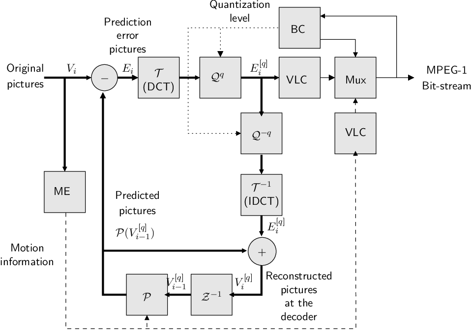
2.3.3.3: The hybrid video encoder

In the figure above we see the hybrid video encoder. For encoding I-frames, we do a DCT + quantization. This compressed frame is then coded using entropy-coding and is then ready. The frame is also fed to a reverse DCT + quantization and put in a frame buffer for predicting the P-frames. When encoding P-frames, we get a new frame from the raw video, and compute the residual between this frame and the previous I-frame. We then do a DCT + quantization on this followed by entropy coding, and we have one of the two parts for the P-frame. We also find the motion vectors needed to transform the previous I-frame into the current frame. These are caulculated, and then entropy coded.
2.4: Quality measures
2.4.1: Objective measures
Image quality can be assesed objectively by SNR or PSNR
Objective measures has some weaknesses. For example if we have one corrupted line, the PSNR will still be high, while most people would not see this as a good image. A tilt in the image will result in a low PSNR, while it would not be noticable for people.
2.4.2: Subjective measures
Determined based on the judgement of a large number of viewers and after elaborate tests comparing the reference and modified content. Results are summarized using mean opinion scores (MOS).
Some weaknesses of subjective measurements is that the viewing conditions may not be optimal, so that the focus may be on the outer things rather than the content to be tested
Part 3: QoE
3.1 QoE:
Quality is defined by ISO9000 as "The degree to which a set of inherent characteristics fulfulls requirements" ITU-T defines it as "The overall acceptability of an application or service, as percieved subjectively by the end-user" Qualinet defines QoE as "... The degree of delight or annoyance of the user of an application or service. It results from the fulfillment of his or her expectations with respect to the utility and/or enjoyment of the application or service in the light of the users personality and current state." phew..
The difference between QoE and QoS is shown in the below table || QoS || QoE || || Network-centric || User centric || || Delay, packet loss, jitter || Content dependant || || Transmission quality || Context dependant || || Content agnostic || Perception ||
QoE sets the user in focus, and as we know, users are not a homogeneous group.
3.2: Universal Multimedia Access (UMA)
The UMA addresses the delivery of multimedia resources under different and varying network conditions, diverse terminal equipment capabilities, specific user or creater prefererences and needs and usage environment conditions. UMA aims to guarantee unrestriced access to multimedia content from any device, through any network, independently of the original content format, with guarantees and efficiently and satisfying user preferences and usage environment conditions. The fulfillment of UMA requires that content is remotely accessible and searchable. Useful descriptions about the content and context (terminal capabilities) are needed. We need content delivery systems able to use this information to provide the intended value to the users independently of location, type of device. One crucial part is the content and context descriptors, which decides if the content needs to adapt before delivered to the end user. MPEG-7 and MPEG-21 are well suited for implementation of UMA-systems
3.3: Immersion
The sene of being immersed, can be described as "being there" when consuming content. The duality in creating an experience is "the sense of realness" or "the sense of being there"
Part 4: Information theory
It is of both practical and theoretical interest to understand how much we can compress any given data source.
In the lossless case this should be some number that tells us that this data source has a representation that is a factor
It would still be valuable to know the absolute limit on how much a data source can be compressed.
For the lossy case we would like to know the compression limit given an allowable amount of distortion. Or vice versa -- how much distortion must we allow if the compression needs to be smaller than some factor
Information theory is the scientific study of the quantification, storage, and communication of information.
- Quantification: We need descriptions of information sources. For this we use statistics, and specify information sources in terms of distributions over alphabets and symbol sequences.
- Storage: How much space is needed to store
$N$ bytes of information from a given source. This is the main topic of our lectures. - Communication: Given a channel with additive noise; what is the capacity in symbols per seconnd, that can be transmitted with an arbibtrarily low probability of error?
The concept of information lies at the heart of Information Theory. We need to be able to specify what we mean by information, and how to measure and quantify it.
When we watch the news, read a book of listen to the radio - we can imagine that we receive information if we learn something we didn't already know. Depending on how long, or how may pages, was needed to convey that information to us, we can sort of say something about how efficiently that information was conveyed.
As a thought experiment we can imagine trying to shorten down a news clip to its bare essentials - just the actual information. How few sentences can one use? When do we hit a limit where using fewer than say
To be able to formalize this process we need to get down to the most basic of information sources - the flip of a coin.
4.1: The Entropy and Data Compression
Information and entropy
Imagine that instead of watching your favorite news show, you are watching a person flip a coin. Altough mundane, the result of such a flip is still information. Watching the coin flip turning up as heads or tails is something you didn't know beforehand.
We assume that a sequence of coin tosses are identically and independently distributed (iid), with probabilities
Pondering
- Assume the probability
$p$ of heads is 1.0. How much information do you think you get by observing heads after a toss?- A good guess would be zero. Since we know that the toss is going to be heads the information we get when it happens is nothing.
- How much information would you receive if a toss with the same coin yielded tails?
- If something is impossible, the corresponding information should be infinite. Informally, if we have coins with probabilities 1/10, 1/1000, 1/1000000 and so on for getting heads, we would think the smaller odds yields more information. As
$p\rightarrow 0$ the informastion should grow to infinity.
- If something is impossible, the corresponding information should be infinite. Informally, if we have coins with probabilities 1/10, 1/1000, 1/1000000 and so on for getting heads, we would think the smaller odds yields more information. As
- If two coins have
$p$ equal to 0.1 and 0.5 respectively, which coin would yield the most surprising tosses on average?$p=0.1$ yields more information, but happens more rarely.$1-p=0.9$ is less informative and happens more often. Although we cannot say for sure just yet, intuition tells us that coin tosses with$p=0.5$ is more informative on average.
- If you toss two coins independently, what should the average information be when compared to a single toss?
- Two independent coin tosses should yield double the information that a single coin toss should. With fair coin, seeing eg. {heads,heads} has a probability of 1/4, while just seing heads for a single, fair coin toss is 1/2.
We want a measure of information that is expressed as a function
$f(1) = 0$ . Things that are sure yields no information$f(0) = \infty$ . Impossible outcomes have infinite information$f(p_1,p_2) = f(p_1)+f(p_2)$ if tosses are independent
The function that makes all three constraints hold is
\begin{equation} f(p) = \log_2(p) = \frac{\log p}{\log 2} \end{equation}
The reason for using the 2-logarithm is that we want to measure information in bit.
Having defined a measure of information we can introduce the most important quantity in information theory -- the Entropy.
This is defined as the expected, or average, information for an information source, and is defined as
\begin{equation} H(p) = -p \log_2 p -(1-p)\log_2 (1-p) \end{equation}
for the coin toss, or more generally, the binary distribution.
In general, for a finite, discrete random variable
\begin{equation} H(X) = - \sum_i p_i \log_2 p_i = E\left[ -\log_2 p_i \right] \end{equation}
where
Data compression
Before we look at the properties and extensions of the entropy, we state what is to us the most important result regarding the entropy of an information source -- Data Compression.
We need some definitions before we make any statements about data compression. Let
\begin{align} P(X=0) &= p \ P(X=1) &= 1-p \end{align}
Assume that
This is a prefix-code, which means that no codeword is the prefix of another codeword, hence, a coded sequence can be uniquely decoded.
Example. Let ut code the bit sequence 101101001001 using our new code: \begin{equation} 101101001001 \rightarrow 110-111-10-0-110-10 \end{equation}
We seem to have coded a 12 bit sequence into a 14 bit sequence, which doesn't make much sense from a compression perspective. However, another sequency like 000010001000 is coded like
Let
The expected length of a code given a distribution over
\begin{equation} L = E_{X^n}[l(x^n)] = \sum_{x^n} P(X^n = x^n)l(x^n) \end{equation}
4.1.1: Data Compression Theorem
Let
Let's use a concrete example to show the power of this theorem. Let
We compute the entropy of
p = 3/4
H = -p*np.log2(p) - (1-p)*np.log2(1-p)
print("The entropy is", H, "vs the code rate", L/2)
The theorem now tells us that we can find an
The theorem doesn't tell us how to find these codes, or even how large
4.1.1.1: Proof of the Data Compression Theorem (DCT)
We will not give a full, formal proof of the theorem as we would need to introduce a lot of mathematical concepts that you would otherwise have no use for. We will instead give a rough sketch that hopefully gives some insight into the material. For those interested, you should consult chapter three of Elements of Information Theory by Cover and Thomas for a proper proof (online edition available through the NTNU Library).
The main observation behind the DCT is that the set of all sequences of

Formally we say that a sequence is typical if
\begin{equation}
2^{-n(H(X)+\epsilon)} \leq P(x_1,x_2,\ldots,x_n) \leq 2^{-n(H(X)-\epsilon)}
\end{equation}
and we denote the set of all typical sequences as
Let us look at the lower bound
In the same way we can write
so
We see that the sequences defined by the bound are exactly the sequences with roughly
You can now show that the size of the typical set is
We know that we need at least
This means we only need
What about the non-typical sequences then? Again, "it can be shown" that
which means that non-typical sequences are extremely unlikely and can be represented with
4.1.2: Further properties of the entropy
The Joint Entropy
Given two random variables
The Conditional Entropy
Given two random variables
The Chain rule for entropy
From probability theory we know that the joint distribution
We can now easily show that
4.1.3: Huffman codes
We will now present one method to find a set of codes for a set of sequences
The algorithm goes as follows:
-
Find the two symbols with lowest probability (here
$X=$ 4 and 5) -
Assign a 0 and 1 one to each of the symbols
-
Sum their probabilities and insert a new symbol (4,5) into the sorted table
-
Repeat the procedure with symbols
$X=$ 2 and 3, getting a new symbol (2,3) - At the third step we assign 0 to (4,5) and 1 to
$X=1$ , and get a new symbol ((4,5),1) - At the final step we assign 0 to ((4,5),1) and 1 to (2,3)
Pondering
- Is this a prefix code?
- Yes, symbals can be uniqly identified
- What is the average length of a coded symbol for this code
- 2.3
- What is the entropy of the source
$X$ ?- 2.29
- Create a Huffman code for the alphabet
$\{1,2,3,4\}$ with probabilities$P=\{1/2, 1/4, 1/8, 1/8\}$ . Compute entropy and average code length.
4.1.4: Bounds on code length
It can be shown (see chapter five in Elements of Information Theory by Cover and Thomas) if you want some proper proofs), that the optimal code lengths for an information source
\begin{equation} l_i^{\star} = -\log_2 P(x_i) \end{equation}
if we just could use code words of non-integer length that is. Instead we have to use code words with length
\begin{equation} l_i = \lceil -\log_2 P(x_i) \rceil \end{equation}
(Here
We can show the following bound on code lengths,
4.1.5 The Kullback-Leibler divergence (relative entropy)
We will now introduce a very important quantity, both in the field of Information Theory and Statistics. The Kullback-Leibler (or KL) divergence is a measure of how much a distribution differs from a reference distribution, and is defined as
Some important properties of the KL divergence are
- We always have that
$D(P\|Q) \geq 0$ $D(P\|Q) = 0$ iff$P=Q$ .- It is asymmetric, that is,
$D(P\|Q) \neq D(Q\|P)$ in general - If
$H(P,Q)$ is the cross entropy of$P$ and$Q$ , and$H(P)$ is the entropy of$P$ (which is the same as the cross-entropy of P with itself) then$D(P\|Q)=H(P, Q)-H(P)$ .
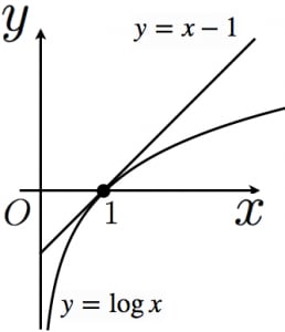
We will quickly prove the first two properties. The third property can easily be proven by finding a suitable example. Before proving (1,2) we need the following inequality
\begin{equation} \log x \leq x - 1~\forall x \end{equation}
Proof
A quick plot is given below in stead of a proper proof.
We can now prove properties 1 and 2 (I will use the natural logarithm in the proof for simplicity. This does not affect the result):
The if part of property 2 is trivially true since
\begin{equation}
\log\frac{P(x)}{Q(x)} = \log 1 = 0
\end{equation}
if
4.1.5.1: Example of the usage of the KL divergence
Assume that we have an information source
for instance by using Huffman coding. We can now give an estimate of how far we will be from the true optimal coding rate,
4.1.6: The Mutual information
The last informastion theoretic quantity we will discuss is the mutual information. It is a quantity used with joint distributions
Let us list some properties of the mutual information before further discussion
4.1.7: The Data Processing Inequality
We now give an application of the mutual information. The Data Processing inequality say that no amount of data processing can improve the inference based on the data.
Before we state the inequality, we need to define a Markov chain. Let
\begin{equation} P(x_k|x_{k-1},x_{k-2}\ldots) \end{equation}
be the probability of
\begin{equation} P(x_k|x_{k-1},x_{k-2}\ldots) = P(x_k|x_{k-1}) \end{equation}
for all
Now consider the Markov chain
Examples:
$X$ is a communication signal (zeros and ones) and$Y$ is$X$ plus some additiver noise$X$ is a label from the set {Cat, Dog, Horse, Capybara}, and$Y$ is a blurry image of the animal
The Data Processing Inequality now states: If we have a Markov chain
Again - this means that no amount of processing of the data
4.1.8: The Entropy rate
The concept of entropy is not limited to iid. random variables, but can also be defined for stochastic processes. Let
\begin{equation} H({\cal X}) = \lim_{n\rightarrow\infty} \frac{1}{n}H(X_1,X_2,\ldots,X_n) \end{equation}
if the limit exists. Examples:
If iid. random variables
We are now read to consdider coding of arbitrarily long sequences.
4.1.9 Differential Entropy
Let
The definition of the differential entropy can be motivated from the discrete entropy as follows:
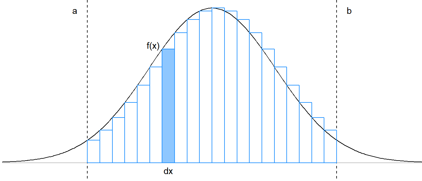
Let
We see that as
This is the reason we refer to
We can define the joint and conditional entropies in the same way as for discrete rvs.
We can also define the continuous versions of the Kullback-Leibler divergence and the Mutual Information:
Because of the linearity of the integral, all the relationships between entropy, joint entropy, conditional entrop
Example 1:
The differential entropy of a zero-mean normal distribution
Example 2:
We can discuss this independently of the underlying distribution. Let
In other words, the entropies of rvs.
4.1.10: Run-length Coding
4.1.11: Arithmetic coding
4.1.12: Lempel-Ziv (LZW) coding
Lempel-Ziv (LZ) codes are widely used for universallossless compression. Due to flexible adaptation mechanisms, these are in principle applicable for compression of any kind of digital data.
Properties of different entropy-coding methods:
| Codewords | Source vectors, fixed-length | variable-length |
| fixed-length | Fixed-length coding (FLC), systematic VLC with 'escape' condition | Run-length coding with FLC, Lempel-Ziv coding |
| variable-length | Shannon & Huffinan coding, systematic VLC with 'typical' condition | Run-length coding with VLC, arithmetic coding |
4.1.13: Vector Quantization
4.2: Rate Distortion Theory
There is a fundamental tradeoff between rate and distortion. This is given by the rate-distortion function. We have previously discussed lossless coding/compression in some detail, and seen that there exists absolute bounds on the performance achievable for a given information source in terms of its entropy.
A natural question is if there exists similar results for lossy compression. The short answer is - yes, but we need some definitions before we can formalize the theory.
We define a distortion function or distortion measure as a mapping
\begin{equation}
d:{\cal X}\times{\cal \hat X} \rightarrow\mathbb R^{+}
\end{equation}
where
for discrete binary symbols, and the squared error distortion
\begin{equation} d(x,\hat x) = \|x - \hat x\|^2\ \end{equation}
for real numbers.
We can define the distortion between sequences
\begin{equation} d(x^n,\hat x^n) = \frac{1}{n}\sum_{i=1}^n d(x_i,\hat x_i) \end{equation}
We define the
an a decoding function
We can the write the expected distortion associated with the
We are now almost in a position to define the Rate Distortion function
4.2.1: Rate-distortion pair
Definition: A rate distortion pair (R,D) is achievable if there exists a sequence of
4.2.1: Rate-distortion region
Definition: The rate distortion region is the closure of of the set of achievable rate distortion pairs

4.2.3: Rate distortion function
Definition: The rate distortion function is the infimum over all
This definition of the rate distortion function, though intuitive, is highly abstract and not constructive. We will now give a more concrete definition of the rate distortion function
We see that the mapping from
Definition: The rate distortion function
Definition: The rate distortion function
The rate distortion theorem states that
4.2.4: Examples
4.2.4.1: Binary source
The rate distortion function for a binary source
Proof: We can easily prove this using a series of inequalities that we later show are tight for a concrete distribution
We wish to calculate
We start by computing the mutual information when
We now show that the inequality is tight if we choose the conditional distribution
we get the equality

Equality is achieved by choosing
import numpy as np import matplotlib.pyplot as plt
def H(p):
    return -p*np.log2(p) - (1-p)*np.log2(1-p)

def R(D,p):
    R = H(p) - H(D)
    R[ p < D] = 0
    return R

p = 1/2
D = np.linspace(1e-12,1-1e-12,100)

fig, ax = plt.subplots()
ax.plot(D,R(D,p),label="p={}".format(p))
ax.grid()
ax.set_xlabel("Distortion D")
ax.set_ylabel("Rate R")
ax.legend()
4.2.4.1: Continues source
We now look at the rate distortion function corresponding to a Gaussian source \begin{equation} X \sim {\cal N}(x;0,\sigma^2) \end{equation}
We have already show the rate distortion function for a continuous rv. with squared error distortion measure to be
We won't show how to compute
We plot the function below
sigmasq = 1.0
D = np.linspace(1e-6, 2*sigmasq,10000)
R = np.maximum(0.5*np.log(sigmasq/D),0)

fig, ax = plt.subplots()
ax.plot(D,R)
ax.grid()
ax.set_xlabel("Distortion D")
ax.set_ylabel("Rate R")
Two observations:
- The rate
$R=0$ for distortion$D > \sigma^2$ . This makes sense as just coding any sample from$X$ as zero will yield an average distortion of$D=\sigma^2$ - The rate
$R\uparrow\infty$ as$D\downarrow 0$ . Again, this makes sense as we need an infinite number of bits to represent a real number.