# Complex numbers "A complex number is a number that can be expressed in the form $a + bi$, where $a$ and $b$ are real numbers and $i$ is the imaginary unit" -wikipedia.org $$ i = \sqrt{-1} $$ $$ i^2 = -1 $$ $$ Re(a + bi) = a $$ $$ Im(a + bi) = b $$ ## Modulus Essentially the length of the vector from the origin to $(a, b)$. $$|w| = |a + bi| = \sqrt{a^2 + b^2}$$ ## Argument The line from the origin to (a, b) has an angle $\theta$. This is called the argument and is denoted by arg $\theta$. The _principal_ argument Arg $\theta$ (with the _initial letter capitalized_) is the value in the interval $(−\pi, \pi]$ ## Polar form Given $r = |w|$ and $\theta = arg\:w$ $$w = r\:cos\:\theta + i\:r\:sin\:\theta$$ ## Multiplication $$ |wz| = |w||z| $$ $$ arg(wz) = arg(w) + arg(z) $$ ## Division $$ \left|\frac{z}{w}\right| = \frac{|z|}{|w|} $$ $$ arg\left(\frac{z}{w}\right) = arg(z) - arg(w) $$ ## Complex form Euler's formula: $$ e^{ i\theta } = \cos \theta + i\sin \theta $$ Based on that formula, we can write a complex number $w$ in complex form. $$r = |w|$$ $$\theta = Arg\;w$$ $$w = r\,e^{i\theta + 2 \pi i k} = r\,e^{i(\theta + 2 \pi k)}$$ where $k = 0, \;\pm 1, \;\pm 2, \;\dots$ ## Roots When finding the $n$th roots of a complex number $w$, we can find $n$ roots. These $n$ roots are distinct complex numbers. For example, let's find $\sqrt[3]{w}$ where $w = 4 + 4i$. We expect to find 3 roots. First, write $w$ in complex form: $$ r = |w| = \sqrt{4^2 + 4^2} = \sqrt{32} $$ $$ \theta = arg(w) = tan^{-1}\left(\frac{4}{4}\right) = \frac{\pi}{4} $$ $$ w = \sqrt{32} \: e^{i(\pi/4 + 2 \pi k)} $$ where $k = 0, \;\pm 1, \;\pm 2, \;\dots$ Next comes the most important step: raise both sides to the power of $\frac{1}{3}$: $$ w^{\frac{1}{3}} = \left(\sqrt{32} \: e^{i(\pi/4 + 2 \pi k)} \right)^{\frac{1}{3}} $$ $$ \sqrt[3]{w} = \sqrt{32}^{\frac{1}{3}} \: e^{\frac{1}{3} i(\pi/4 + 2 \pi k)} $$ Finally insert $k = 0, 1, 2$ to get the three 3rd roots of $w$ respectively. Note: If you try to insert $k = 3$, you'll see that it gives the same root as $k = 0$ ## Complex functions $$ \cos{z} = \frac{e^{iz} + e^{-iz}}{2} $$ $$ \sin{z} = \frac{e^{iz} - e^{-iz}}{2i} $$ # Second order linear differential equations ## Linear, homogenous equations with constant coefficients $$ y''+py'+qy=0 $$ Solve $\lambda^2+p\lambda+q=0$ ### Distinct real roots $$y(t)=C_1 e^{\lambda_1t}+C_2 e^{\lambda_2t}$$ Where $C_1$ and $C_2$ are arbitrary constants. ### Complex roots $$z_1(t)=e^{(a+ib)t}=e^{at} [cos(bt) + i sin(bt)]$$ $$z_2(t)=e^{(a-ib)t}=e^{at} [cos(bt) - i sin(bt)]$$ $$y(t)=C_1z_1(t)+C_2z_2(t)$$ ### Repeated roots $$\lambda=-p/2$$ $$y_1(t)=e^{\lambda t}$$ $$y_2(t)=te^{\lambda t}$$ $$y(t)=(C_1+C_2t)e^{\lambda t}$$ ## Inhomogeneous equations The inhomogenous linear equation $$ y''+py'+qy=f $$ Has the general solution: $$ y=y_p+C_1y_1+C_2y_2 $$ Where $y_1$ and $y_2$ are solutions to the associated homogenous equation $$ y''+py'+qy=0$$ and $y_p$ is a particular solution to the inhomogenous equation $$ y''+py'+qy=f$$ # Vectors A vector in this subject is always thought of as a column vector, and is written as such: $$ \vec{v} = \begin{bmatrix} v_1 \\ v_2 \\ \vdots \\ v_n \end{bmatrix} $$ ## Normalization of vectors When we normalize a vector we are making the length of the vector $1$ (for the zero vector, with length equal to zero, this is not possible). This is an important operation in regards to steady-state vectors and computer graphics. A normalized vector is also called a unit vector. $$ \vec{\hat{v}} = \frac{\vec{v}}{\begin{Vmatrix} \vec{v} \end{Vmatrix}} $$ Where $\begin{Vmatrix}\vec{v}\end{Vmatrix}$ is the length of the vector: $$ \begin{Vmatrix}\vec{v}\end{Vmatrix} = \sqrt{v_1^2 + v_2^2 + \dots + v_n^2}$$ # Matrices ## Terminology For example, when a text says _"Suppose a 4 x 7 matrix A (...)"_, that means that _m_ = 4, _n_ = 7. Can't remember the order? Rule of thumb: Just remember the word "man" and that _m_ comes before _n_. _m_ is the height of the matrix, and _n_ is the width of the matrix. ## Linear transformations A matrix can be regarded as a transformation that transforms a vector. For example, a transformation $T$ can double the length of a 2D vector. Such a transformation $T$ and its standard matrix $A$ would look like this: $$ T(x) = 2x $$ $$ A = \begin{bmatrix} 2 & 0 \\ 0 & 2 \end{bmatrix} $$ ### Onto and one-to-one Let $A$ be the standard matrix of a transformation $T\; : \; \mathbb{R}^n \; \rightarrow \; \mathbb{R}^m$ - $T$ is _onto_ if and only if the columns of $A$ span $\mathbb{R}^m$. In other words, $Ax = b$ has a solution for each $b$ in $\mathbb{R}^m$. - $T$ is _one-to-one_ if $A$ is invertible, i.e. the columns of $A$ are linearly independent. ## Inverse of a matrix The inverse of a matrix $A$ is denoted $A^{-1}$ and is the matrix that one can multiply A with to get the identity matrix. $$ A^{-1}A = I $$ For example, consider the following matrix $$ A = \begin{bmatrix} 2 & -1 & 0 \\ -1 & 2 & -1\\ 0 & -1 & 2 \end{bmatrix}. $$ To find the inverse of this matrix, one takes the following matrix augmented by the identity, and row reduces it as a 3 by 6 matrix: $$ [\;A\;|\;I\;] = \left[ \begin{array}{rrr|rrr} 2 & -1 & 0 & 1 & 0 & 0\\ -1 & 2 & -1 & 0 & 1 & 0\\ 0 & -1 & 2 & 0 & 0 & 1 \end{array} \right]. $$ By performing row operations, one can check that the reduced row echelon form of the this augmented matrix is: $$ [\;I\;|\;B\;] = \left[ \begin{array}{rrr|rrr} 1 & 0 & 0 & \frac{3}{4} & \frac{1}{2} & \frac{1}{4}\\[3pt] 0 & 1 & 0 & \frac{1}{2} & 1 & \frac{1}{2}\\[3pt] 0 & 0 & 1 & \frac{1}{4} & \frac{1}{2} & \frac{3}{4} \end{array} \right]. $$ By this point we can see that B is the inverse of A. A matrix is invertible if, and only if, its determinant is nonzero. ## LU factorization With this technique, you can write $A = LU$ where $L$ is a __l__ower triangular matrix with ones on the diagonal and $U$ is an __u__pper triangular matrix (echelon form). Do this only if you can reduce A without row exchanges. First, write down the augmented matrix: $$ [\;A\;|\;I\;] $$ Row reduce it until the left side is in _echelon form_ (not reduced echelon form). You should now have $$ [\;U\;|\;L^{-1}\;] $$ Now, to find L, use your favorite technique for finding the inverse of a matrix. __Why LU factorization?__ Because when $A = LU$, and you want to solve $Ax = b$ for $x$, then you can find $x$ by solving these two equations: $$Ux = y$$ $$Ly = b$$ Each of these two equations are relatively simple, and computers are able to solve them faster than solving the more complex equation $Ax = b$ ## Determinants The determinant of a 2x2 matrix is simple to compute. Here's an example: $$ A = \begin{bmatrix} a & b \\ c & d \end{bmatrix} = \begin{bmatrix} 4 & 9 \\ 3 & 2 \end{bmatrix} $$ $$ det\: A = ad - bc = 4 * 2 - 9 * 3 = -19 $$ Calculating the determinant of a larger matrix is harder. Look up "cofactor expansion" in your textbook or on the internet. Moreover, here are some useful theorems related to determinants: - If $A$ is a triangular matrix, then $det\: A$ is the product of the entries on the main diagonal of $A$. - Adding one row of $A$ to another row of $A$ will not change $det\: A$. - A square matrix $A$ is invertible if and only if $det\: A \neq 0$. ## Eigenvalues and eigenvectors Eigenvalues and eigenvectors apply to square matrices. ### Eigenvalue #### Definition An eigenvalue is a value that satisfies this equation: $$ A \vec{v} = \lambda \vec{v} , \vec{v} \neq 0 $$ To find the eigenvalues you evaluate the definition. $$ A \vec{v} = \lambda \vec{v} $$ $$ A \vec{v} - \lambda \vec{v} = 0 $$ $$ (A - I \lambda) \vec{v} = 0$$ This is where $I \lambda$ is the identity matrix of $\lambda$. To satisfy $\vec{v} \neq 0$ we need to make sure the determinant to $A - I \lambda$ is equal to zero. This will yield a polynomial equation, which when solved will give the eigenvalues. #### An example of finding the eigenvalues of a matrix Given the matrix: $$ A = \begin{bmatrix} 1 & 2 \\ 4 & 6 \end{bmatrix} $$ We want to find the eigenvalues. We have from the definition that the eigenvalues satisfies this equation: $$ \begin{vmatrix} A - I \lambda \end{vmatrix} = 0 $$ We then have: $$ \begin{vmatrix} 1 - \lambda & 2 \\ 4 & 6 - \lambda \end{vmatrix} = 0 $$ Which then gives the polynomial $$(1-\lambda)(6-\lambda)-8=0$$ $$\lambda^2 -7\lambda-2=0$$ The roots of this polynomial are $\frac{1}{2}(7-\sqrt{57})$ and $\frac{1}{2}(7+\sqrt{57})$, which are the corresponding eigenvalues of $A$. ### Eigenvectors After we have found the eigenvalues, we can find the eigenvector. The eigenvectors are the vectors that satisfy the equation: $$(A-I\lambda)\vec{v}=0$$ Where $\lambda = {\lambda_1, \lambda_2, ..., \lambda_n}$. ### 2D rotation matrix Given that $a$ and $b$ are real numbers, $C$ is a 2 x 2 transformation matrix that scales and rotates a vector. $$ C = \begin{bmatrix} a & -b \\ b & a \end{bmatrix} $$ The eigenvalues of $C$ are $\lambda = a \pm bi$ and the scaling factor of $C$ is $r = |\lambda| = \sqrt{a^2 + b^2}$ Then $C$ can be rewritten like this: $$ C = r \begin{bmatrix} a/r & -b/r \\ b/r & a/r \end{bmatrix} = \begin{bmatrix} r & 0 \\ 0 & r \end{bmatrix} \begin{bmatrix} \cos \varphi & -\sin \varphi \\ \sin \varphi & \cos \varphi \end{bmatrix} $$ where $\varphi$ is the angle of the transformation $C$ ## Column Space and Null Space of a Matrix The __column space__ of a matrix A is the set Col A of all linear combinations of A. The vector $\textbf{b}$ is a linear combination of A if the equation $A\textbf{x} = \textbf{b}$ has a solution. If $V$ is a vector space, then $dim\: V$ is the number of vectors in a basis for V. __Rank A__ = dim Col A The __null space__ of a matrix A is the set Nul A of all solutions of the homogeneous equation $A\textbf{x} = \textbf{0}$ ### Basis

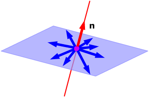
## Orthogonality A set of vectors is orthogonal if the vectors in the set are orthogonal (perpendicular) to each other. Two vectors $u$ and $v$ are orthogonal to each other if $u \cdot v = 0$. In other words, $u^T v = 0$ ### Orthogonal complement The set of all vectors $z$ that are orthogonal to $W$ is called the orthogonal complement of W and is denoted by $W^{\perp}$. $W$ is a subspace of $\mathbb{R}^n$, for example it is a plane in $\mathbb{R}^3$. The orthogonal complement of that plane would be the normal vector to that plane. Here's another example: If $W$ is a line in $\mathbb{R}^3$, then $W^{\perp}$ is the plane that is perpendicular to the line.  ### Orthonormal set An orthonormal set is orthogonal, but has one extra requirement: Every vector has length equal to 1. If you construct a matrix $U$ with the vectors of an orthonormal set as columns, then $U^T U = I$. Why? Because matrix multiplication can be regarded as a set of dot product operations. Each column in $U$ dotted with any other column in $U$ will become zero, but a column in $U$ dotted with itself will become one. This also means that $U^{-1} = U^T$ if $U$ is square. ### QR factorization If $A$ is an m x n matrix with linearly independent columns, then $A$ can be factored as $A = QR$. $Q$ is an m x n matrix whose columns form an orthonormal basis for $Col\:A$. $R$ is an upper triangular invertible matrix with positive entries on its diagonal. You can use Gram Schmidt for finding $Q$. 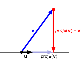When finding R, you can use the fact that the columns of $Q$ are orthonormal, and thus $Q^T Q = I$: $$ A = QR $$ $$ Q^T A = Q^T Q R $$ $$ Q^T A = I R $$ $$ R = Q^T A $$ ### Projection $\hat{y}$ is the vector $y$ projected down to the line $L$ spanned by the vector $u$ $$ \hat{y} = proj_L y = \frac{y \cdot u}{u \cdot u} u $$  ## Symmetric matrices A symmetric matrix is a square matrix $A$ such that $A^T = A$. For any symmetric matrix $A$, this is true: $A^T A = A A^T$ If $A$ is symmetric, then any two eigenvectors from different eigenspaces are orthogonal. # Useful links [Recap lecture (Norwegian)](http://multimedie.adm.ntnu.no/mediasite/Catalog/catalogs/ekm3.aspx) [Course videos (Norwegian)](http://video.adm.ntnu.no/openVideo/serier/4fe2d4d3dce25) [Second order differential equations on Khan Academy](https://www.khanacademy.org/math/differential-equations/second-order-differential-equations) [Linear algebra on Khan Academy](https://www.khanacademy.org/math/linear-algebra) [Official website with homework assignments, old exams etc.](https://wiki.math.ntnu.no/tma4115)