‹

CS-450: Advanced algorithms

Tags:

Algorithms

Introduction

This compendium is made for the course CS-450 Advanced Algorithms at École Polyteqnique Fédérale de Lausanne (EPFL) and is a summary of the lectures and lecture notes. Is is not the complete curriculum, but rather a list of reading material.

Professor: Moret Bernard

Course website: http://lcbb.epfl.ch/algs16/

Three tests during the semester counts towars the final grade. Homework every week, but is only for feedback.

Algorithm analysis and design.

Algorithms Analysis
- Fast reminders about worst-case analysus, & asymptotic notation
- Amortized, competitive, randomized analysis
Algorithms design
- Design strategies
  - greedy
  - divide and conquer
  - iterative improvement
  - dynamic programming
- (but implement in a different way, randomized, sampling, projections)

Algorithm analysis

Asymptitic notation

$f(n)$ is in $O(g(n))$ iff $\exists N$ s.t. $\forall n \geq N$. This is an a.e. (upper bound)

a.e.: almost everywhere
- There exist a bound where this is always true.
i.o.: infinitely often
- Only needs another example. This is good for lower bounds

Wagner's conjection: Given a family of graphs defined by a property P. If P is closed under subgraphs and edge contraciton then there exists a finite set of "obstruction" graphs, s.t. every graph not in family includes an obstruction (we can test in polynomial time whether the graphs belogns to the family or not).

An algorithm was also given to find this, which runs in time $c*g(n)$ where $g(n)$ is a $n$ cubed. The probles is that $c$ is of order $10^{1000}$. Conclusion; big-oh can be misleading.

Kuratowski's theorem: A graph is planar iff it does not include one of $K_5$ or $K_{3,3}$

Example:

P: Can be embedded in 3D without knots. Was believed to be impossible, but Wagner's conjection tells us that this can be solved in polynomial time.

Worst-case analysis

Ex. Merge sort: $t(n) = 2t(n/2) + \Theta(n)$. $t(n)$ is in $\Theta(nlogn)$.

Be able to solve reccurence relations!!

Amortized analysis (connected with data structures)

Look at the cost of a sufficiently long sequence of operations. Do worst-case analysis on sequences of operations (of unknown lenght)

Standard tool: A potential function

Ex: Stacks; push and pop

How many operations is sufficient to calculate amortized? Max $n$ operations. $\Phi_{final} - \Phi_{initial}$. If the running time is $\log n$, then we need a sequence of at least length $\frac{n}{\log n}$. A smarter potential function could give the same running time, but give a smaller sufficient lenght of the sequence.

Add a new operation: "empty", but this has to be implemented as pop'ing as long as there are elements left.

Claim: If we start with an empty stack, then any sequence of $n$ operation takes $\Theta(m)$ time.

$\Phi(stack) = sizeofstack$ where $\Phi$ is the potential function.

Push, pop and empty takes some time and also modify the potential function.

	time	$\Delta \Phi$
Push	1	-1
Pop	1	+1
Empty	$\Phi(stack)$	-$\Phi(stack)$

Example:

Incrementing a binary integer: Worst-case $O(log(n))$.

Amortized: $K(k$ large with respect to $n$) incrementations take $O(k)$ fi you take it over a sequence of k operations.

Design of potential: We want a simple potential function. Instead of counting trailing 1's, we can simplify and take to number of 1's in the binary representation.

Increment $n$.

Yes, you had to do a lot of work, but this made the number nice for further incrementations. It improves the state of the structure.

cost	$\Delta \Phi$	sum
i	1 - (i - 1) = 2 - i	2 (constant)
j	$\Phi_{j+1} - \Phi_j$
j+1	$\Phi_{j+2} - \Phi_{j+1}$
j+2	$\Phi_{j+3} - \Phi_{j+2}$

$$ \sum_{j=1}^k cost_j + \Phi_{k+1} - \Phi_0 = 2K $$ $$ \sum_{j=1}^k cost_j = 2K - (\Phi_{k+1} - \Phi_0) $$ $$ \sum_{j=1}^k cost_j = 2K + \Phi_0 - \Phi_{k+1} $$

$$ \sum_{j=1}^k cost_j \leq 2K + \Phi_0 - \Phi_{k+1} $$

$\Phi$ can never be greater than of order $n$, so $k$ dominates.

$$ 0 \leq \Phi_i \leq \log n $$

For $k \in \Omega(\log n)$ a sequence of $k$ incr. on $n$ takes $O(k)$ time.

Amortized data structures

Does not try time give a worst-case guaranty, but will give a worst-case over $k$ operations.

Example: priority queue:

Insert (item, priority)
Delete min.

Binary heap:

Guaranty heap property: Priority of the parent is better (i.e. smaller) than the priority of the children. Delete takes at max $\log n$. Merging two trees is at best linear time. We want meldable priority queue (mergable).

Leftist tree:

Binary tree, obeying the heap property & it has the leftist property, i.e. the shortest path to a leaf from an internal node is on the right. The consequence is that the tree leans to the left.

THe right edge can at most have lenght $\log n$ of decreasing priority.

How to merge two trees in $\log n$?

We just have to merge the two right paths. We can rotate the tree (see wikipedia article linked in this header). We can merge teh top part (the right siden in the unrotated one) as two sorted lists. Takes $O(\log(n_1) + \log(n_2))$ time. The result is not neccesarily leftist. The problem is that the child trees have to be sorted in increasing height. There is no smart way of doing this except from storing extra information, in practice how far is it to the closest leaf. Each node stores dist. from it to closest leaf.

Hand-note

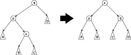
Delete min:

Behead the tree. How long time does this take? As the frenchmen found out during the revolution, is very easy, constant time!!! - Our French professor

Then we can just meld the two child trees.

Amortized:

When merging trees, instread of keeping track of length to leaf node we can always swap the children instead. This will give just as good time, but amortized. If you do nothing, you double the lenght of the path.

Claim: amortizes to $O(\log n)$ time per operation.

Design a potential function:

How far is it from a leftist tree? This gets a bit complicated.

We can try to define the potential as $w(x) = \#descendants$. The bigger the tree is, the greater the chance of the lenght of the right side is longer.

If $w(y) < w(x) \rightarrow bad$. What if $w(y) = w(x)$

$\log n$ is all I'm after - Professor

$w(x)$ is size of subtree rooted at $x$.

$x$ is heacy iff its weight is larger than $\frac{1}{2}$ weight of its parent.

$\Phi(T) = $ # heavy nodes that are also right children.

If we have a path from $x$ to $y$ famed entirely of light nodes, then the length of that patf is $\leq \log \frac{w(x)}{w(y)}$.

The weigth of whats under the node decreasing by half for every time(binary search).

On any parh from the roow to a leaf, there are $O(\log n)$ light nodes, so heacu nodes are the problem. The right most path is the problem. How does heacu nodes stay or go to the right most part. Because every time we merge we flip the paths.

TODO: Fill in conclusion. A little unclear for me.

cost	$\Delta \Phi$
$rp_1 + rp_2$	$m_l - m_h$

cost is made out of light & heavy nodes, $O \log(n_1 + n_2)$ light nodes. $rp_1 + rp_2 = m = m_l + m_h$ $$ cost + m_l - m_h = 2m_l$$

Sum is $2m_l k $ where $k$ is lenght of the sequence, and $m_l$ is bounded by $\log n$.

Compeatable (<- TODO) algorithms

Splay trees.

KISS: Keep it simple stupid

Think of meldable trees. It has to be some kind of link structure to be melded efficiently. Often trees. KISS. Binary trees.

Either heap-ordered of a sorted inorder.

A binary search tree!

Idea: search($x$). After the first seach we can then use paging as known from as OS course. Actually, we will move $x$ to the root.

operations of splay($x$):

Move $x$ to the root if $x \in T$ else ?.

If $x$ is root, do nothing.

If x is one step down:

If 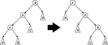$x$ is deeper: Wikipedia

or Wikipedia

splay($x$) on a tree of size $n$ takes $O(\log n)$ amortized time.

What if $x \notin T$. Still move the neighbor to the top. Move either $x^-$ or $x^+$. We still haven't defined any useful operations on the tree. Splay is the same principle as meld. This is the only operation we will use.

All operations defined in terms of splay

All I can do is splay. I'm sorry, I'm not very good at this. - Professor

We can implement this in a smarter way, but the reason to do everything in terms of splay is that the analysis is smoother.

Insert: run splay(x); if root has $x$ done; if not in tree is splay($x$) on $B$ if $B \neq \emptyset$. ($x$ must go in $B$). If we do splay on $B$, then we will get the successor. Put in in the root, and we can easily insert $x$.
Deletemin: Just splay minimum possible key. This will either bring up the smallest possible key or the predeccessor, which is then the smalles key in the tree.

Amortized analysis

$w(x) =$ weight of $x =$ size of subtree rooted at $x$.

$r(x) = \log w(x)$. $r(x)$ is a surrogate for the height.

Cost of splay($x$):

$\leq 1 + 3(r_{after}(x) - r_{before}(x))$.

Rotation $i$ has a cost $\leq 3(r_{i+1}(x) - r_{i}(x))$ and similar for rotation $i + 1$. If we sum all the steps we end up with the final rank in the end minus the original rank. The 1 in the front is only for the first rotation.

$r_{after}$: $r^{'}$
$r_{before}$: $r$
$\Delta \Phi$: $r^{'}(x)$ -$r(x) + r^{'}(y)$ -$r(y) + r^{'}(z)$ -$r(z) \leq 3(r^{'}(x)$ -$r(x))$

We have to sum up real cost and $\Phi$.

$2 - r(x) + r^{'}(y) - r(y) + r^{'}(z)$ Note $r^{'}(x) \> r^{'}(y)$.

TODO: Fill in

What is the max of $\log s + \log t$? $\log s + \log t$ is maximized with $s + t = 1$ and then (calculus) with $ s + t = \frac{1}{2}$. $max(\log s + \log t) = -2$

$2 + r'(x) + r'(z) 2r(x) \leq 3(r'(x) - r(x) = \log \frac{w'(x)}{w(x)} + \log \frac{w'(z)}{w(x)}$

TODO: fill in

laziness is good (for data structures)! - Professor

Lazy leftist tree

Leftist trees that support arbitrary delete. We are prepared to do operations on the right side of the tree, but not in an arbitrary place. The solution is to not delete it, but jusk mark it as deleted.

Deletemin: partial fix. The min node might be dead, so not the min. Fix the top of the tree. Go down to une level under the one taht has alive nodes. We can then get many subtrees and meld them two by two. Cost is $k \log n$

Competitive Analysis

Amortized analysis against an unknown optimal strategy -> so ration instead of absolute values.

Example: Paging strategy LRU (least resently used)

A list that can only be searched sequentially. We can move a used item to the front of the list MTF(move-to-front). We can not do worst time, and it is difficult to do amortized.

We can compare it to the optimal, even though we don't know the optimal strategy.

Claim: MTF does no worse that twice the cost of the optimal strategy.
- SubClaim: MTF does no worse that twice the cost of the static strategy. (But this method can look at all the expected searches and then decide the fixed order).

Alg(1)(unknown): Picks a fixed oridering that is optimal for the sequence of queries to come.
Alg(2): MTF

We will compare the two algorithms and do an amortized analysis.

$\Phi = \sum_{x \in list} \phi(x)$

$\phi(x) = \text{# of elements in front if x in MTF, but behind x in optimal}$

real cost(x) in MTF: i
real cost(x) in optimal: j

	cost(x)	cost(x) + $\Delta \Phi$
MTF:	$i$	$i + (- \phi_x) + 1 \cdot (i - 1- \phi_x) = 2(i - \phi(x)) - 1$
Optimal:	$j$	$2j > 2(i - \phi(x)) - 2$

$2\text{opt} \geq \text{real cost} + \Delta \Phi$

$2 \sum \text{real cost}_{opt} \geq \sum \text{real cost}_{MTF} + \Phi_{final} - \Phi_{initial}$

Example: Dynamic arrays

Array is to small, double it
Array is too large, reduce it
- We need a halving threshold

Randomized analysis

Protection / guerantee against bad distribution of the real data
Yields very simple & very fast algorithms
Higher reliability than deterministic version

Make a deterministic algorithm stochastic to protect against unknown events in the outside world. We cannot do average case, since we can not control the probability distribution of the outside world. The real world is not perfect random.

Problem with for instance quicksort. By providing the randomness ourselves, we get an expected $=(n \log n)$ time regardsless of input sequence.

Analysis of 2d hull

The addition and removal of edges and vertices amortizes to $\Theta(n)$ over algorithm.
The running time is determined by the maintanance of the conflict list structure by backwards analysis.
- What needs to change if we remove the last vertex added. Last vertex is any of the $i$ vertices with equal prob. THe order in which the $i$ vertices were added does not matter.

Karger's algorithm for min cut in a graph

Given a connected, indirected graph, $G=(V,E)$

Def: A cut is a subset of edges whose removal disconnects the graph.

Select an edge on random, with the assumption that this edge is not a part of the graph, since the cut is smalled compared to the total size of the graph. Mincut size is $k$. We know that all vertices has at least $k$ edges (the degree of the vertex). This also tells us that the graph has $\geq \frac{nk}{2}$ edges.

Idea: Pick an edge at random and decide it's not in the cut; modify the graph to reflect that. The edge we have removed does not contribute on disconnecting the graph. Then merge the two end points of the edge. This removes one vertex and one edge. Keep duplicate edges. This is known as multigraph. The size of the min cut has not changed. Repeat this until we only have two vertices. The edges connection these two vertices are the cut.

The probability that we manage to avoid the min cut in the start is good, but as the algortihm runs, the cut size $k$ stays the same but the total amount of edges decreases.

Min cut size $k$
# edges $geq \frac{nk}{2}$
Not hitting min cut at first choice: $1 - \frac{k}{nk/2} = 1 - \frac{2}{n}$
Not hitting min cut at second choice: $1 - \frac{2}{n - 1}$

Probability of geting a mincut at the end:

$$ (1-\frac{2}{n})(1-\frac{2}{n-1}) \dots (1-\frac{2}{3}) = \text{Not so great}$$

Probability is $\frac{2}{n(n-1)}$

Repeat the algorithm $n^2$ times and we end up by a constant probability. We can improve this by running the time $100n^2$ or $1000n^2$. It total this is $n^3$.

This is very robust, very fast and very cute! - Professor

$Pr(x - \epsilon \leq x \leq \bar{x} + \epsilon) \geq 1 - \sigma$

Make assumptions to analyse the tails of deviation.

Markov theorem (Markov inequality):

Probability distribution x with exp. $\bar x$; $pr(x > k \cdot \bar x ) \leq \frac{1}{k}$.

Need more knowledge about distrubution to get tighter bounds. We know the variance and the mean. $Pr(x > \bar x + k \cdot \sigma_x < \frac{1}{k^2}$.

Assume $x$ is the sum of independent variables => Chernoff bound (exponetial bounds)

Proof: Use Markov inequality using exponential generating functions.

Algorithm design

Dynamic programming

Discrete, finite Markoc models.

A collection of states, $S = \{S_1, S_2 \}$
A stochastic transition matrix $T = [t_{ij}]$

$$ \text{Markov model} \equiv \text{stochastic autoomation}$$

Add an output function (emission), also stochastic. If we have finite output alphabet $E = \{c_1, c_2, \dots , c_m \}$ then we also have a right stochastic emission matrix $E_{nm} = [e_{ij}]$. In pratice, many entries of the transition matrix $T$ are set to zero.

Slightly dishonest casino

Dice are supposed to create an equally possible output. You can create a slightly weighted (pipped) die. $\Sigma = \{1,2,3,4,5,6\}$. Two states. One where the casino is using a true dice, and one where they are using a pipped dice.

Baum-Welch algoritm

Written by

Martin Hallén

Last updated: Tue, 5 Apr 2016 09:11:43 +0200 .