ABC123: Personal version of algdat
Are you looking for an overview of all runtimes, you will find them all at the bottom, Runtimes for Curriculum Algorithms.
What are algorithms?
An informal definition: An algorithm is any clearly defined method for calculations that can take a value (or a set of values) as input and return a value (or a set of values) as output.
One can also view it as a tool that can solve a defined calculation problem. When defining the problem, one has to describe which relationship is desired between input and output, for example: «Input: A city road map and two points. Output: The shortest path (measured in meters) between the two points.»
Description of solution: There is no general standard for describing an algorithm. You can describe it with natural language, pseudo code, as code or through hardware drawings. The only requirement is that the description is precise.
Instances: Each collection of input-values to a problem is called an instance. For example can an instance of the problem above have input values such as a road map of Trondheim, and the two points are the geographic coordinates of NTNU Gløshaugen og NTNU Dragvoll.
True or False?: An algorithm can either be true or false. If an algorthim is true, it will for all possible instances defined give the correct output; for example it is only to be expected that a sorting problem will not have problems sorting all possible collections of positibe whole numbers. If it is false, this will not be the case. F.ex: you may have invented an algorithm that solves all sorting problems by returning the list in reverse. This will only in some instances return the correct output, but only for a subset of potential instances.
Basic Data structures
This course covers several different data structures with respect to various problems. It is therefore important to have a general overview of the most important ones.
Linked lists

Singly linked list (Public Domain, Lindisi)
A linked list is a basic linear structure that represents elements in sequence. The concept behind the structure is that the sequence of elements is conserved by each element pointing to the next in the sequence (se the figure above). Explained in code:
class Node:
    def __init__(self):
        self.value = None
        self.next = None

n1 = Node()
n2 = Node()
n3 = Node()
n1.value = 1
n2.value = 2
n3.value = 3
n1.next = n2
n2.next = n3
With the code above the structure will be n1 -> n2 -> n3
We can also have double linked lists, where each node contains a value and a pointer both to the previous and next nodes.
Runtimes
| Action | Runtime |
| Insert at the start | |
| Insert at the end | |
| Lookup | |
| Delete element | lookup + |
Abstract Data structures
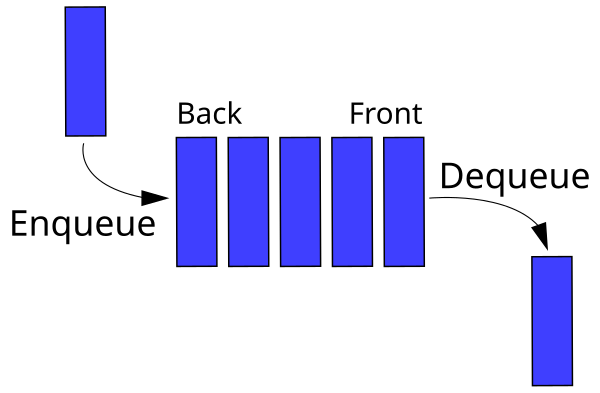
Queue
A queue is an abstract data structure that preserves the elements sequence and has two operations, enqueue and dequeue. Enqueue is the insert function, which inserts elements at the back of the queue. Dequeue is the exctraction function, and retrieves the first element at the front of the queue. A queue is therefore a FIFO-data structure (First In First Out).
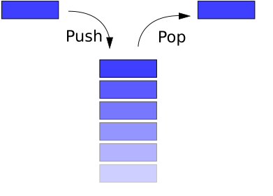
Stack
A stack is an abstract data structure which, similar to a queue, preserves the elements sequence. Unlike a queue however, a stack is LIFO (last in first out) implying that it both inserts and extracts elements from the back of the structure. These operations are called push and pop respectively.
Heap
A heap is a list which can be viewed as a binary tree. A heap is an implementation of the priority tree data structure. Check out heapsort
Max heap property: No node can have a higher value than its parent node.
Hash
The purpose of creating hash tables or (hash maps) is to arrange elements into a predetermined number of groups. Each element passes it's key (this can be it's value) to a hashing function, which determines which group the element is placed in. Multiple elements may be placed in the same group. These collisions aren't inherently bad as they can be dealt with, but may lead to slower run times. Common ways to resolve collisions are by either creating linked lists or using open addressing. The former creates linked lists (chains) for elements with colliding hashes, while the latter moves a colliding element to a different hash. The latter can be achieved with methods like linear probing, quadratic probing, or double hashing.
Bucket sort uses a similar concept to group unsorted elements.
Hash functions
Let
Some hash functions include:
$h(k) = k \;\mathrm{mod}\; m$ $h(k) = floor(m(kA \;\mathrm{mod}\; 1))$ where$0 < A < 1$
To clarify, the first function subtracts
Perfect hashing means that each element is mapped to a unique value. This can be achieved with randomized hashes where
Runtimes
Assuming single, uniform hashing and chaining.
| Function | Best Case | Average Case | Worst Case |
| Lookup |
With a perfect hashing, the lookup only requires you to check the hash and go to it, meaning the time is constant. For a hash table with collisions, the lookup will have to account for the average number of entries in each hash. The worst possible case is that every element is placed into the same hash, requiring a linear search.
Runtime Calculations
Runtime is a measurement of how effective an algorithm is and is by far th emost important measurement in this course.
About Runtimes
In a world where computers are infinitely fast and with unlimited storage space, any true algorithm can be used to solve a problem - no matter how badly designed it was. This is not the case in reality, therefore making runtime an important aspect of programming.
A runtime describes the relationship between the input size and how many calculations (how long time) it takes to solve it. Concider a problem of a known size and with the runtime
Common Runtimes
The following table shows the asymptotic notation for run times. It denotes how the algorithm behaves as
| Name | Notation | Runtime |
| Small-O | ||
| Big-O | ||
| Theta | ||
| Big-Omega | ||
| Small-Omega |
The most general and used runtimes sorted from worst to best.
| Complexity | Name | Type |
| Factorial | General | |
| Exponential | General | |
| Polynomial | General | |
| Cubic | Polynomial | |
| Quadratic | Polynomial | |
| Linearithmic | Combination of linear and polynomial | |
| Linear | General | |
| Logarithmic | General | |
| Constant | General |
Recursion
Recursion is a problem-solving technique which is based on the fact that a solution to a problem consists of the solutions to smaller instances of the same problem. This technique will be a recurring theme in several of the algorithms in the curriculum.
One of the most common examples of recurisivity is the Fibonacci sequence, defined as:
Fibonacci numbers
Examples of recursive algorithms include merge sort, quicksort and binary search. Recursive solutions can also be used in dynamic programming.
The Master Theorem
The Master Theorem is a recipe solution for finding the runtime of several reccurences.
This type of recurrence often occurs together with divide-and-conquer algorithms such as merge sort.
The problem is split up into
If we didn't already know the runtime for Merge sort, we can quickly discover it by solving this recurrence. Solving the recurrence could also be achieved by using the Master Theorem as follows:
- Identify
$a, b, f(n)$ - Calculate
$\log_b a$ - Consult the following table
Table over three potential outcomes of the Master Theorem:
| Case | Requirement | Solution |
| 1 | ||
| 2 | ||
| 3 |
Returning to the merge sort example. We have found
Example
Another example retrieved from the 2009 Continuation Exam:
Solve the following recurrence. Give the answer in asymptotic notation. Give a short explanation.
We have
Sorting and Search
Sorting and search are two problems that either occur as stand alone problems or as a subproblem. Sorting implies organizing a set of elements into a specific order. Searching implies that we are looking to find a certain element in a set of elements.
Search
Finding a specific element in a data structure is a common problem. In a list of numbers we may want to search for the median, or a certain number. In a graph we may want to search for a path from one element to another. Searching algorithms for graphs (DFS and BFS) are covered in Graph algorithms.
The two most common ways to search lists are Brute force and Binary search.
Brute force
This method is pretty self explanatory. Iterate through the list (sorted or unsorted) from beginning to end and compare each element with the element you are trying to find. With
Binary search
If we know that the list we are searching is sorted, we can use a better strategy than brute force. Let
In Python:
def binary_search(li, value, start=0):
    # Dersom lista er tom, kan vi ikke finne elementet
    if not li:
        return -1
    middle = len(li) // 2
    middle_value = li[middle]
    if value == middle_value:
        return start + middle
    elif value < middle_value:
        # Første halvdel
        return binary_search(li[:middle], value, start)
    elif value > middle_value:
        # Siste halvdel
        return binary_search(li[middle + 1:], value, start + middle + 1)
Each iteration will halve the searchable elements. The search can at most take
| Best Case | Average Case | Worst Case |
Sorting
Sorting algorithms can be categorized into two groups: Comparison based and distributed/non-comparison-based.
Stability
A sorting algorithm can be considered stable if the order of identical elements in the list that is to be sorted is preserved throughout the algorithm. Given the following list:
Sorting it with a stable algorithm the identical elements will stay in the same order before and after the sort.
Comparison Based Sorting Algorithms
All sorting algorithms that are based on comparing two elements to determine which of the two are to come first in a sequence, are considered comparison based. It is proven that
Merge sort
Merge sort is a comparison based sorting algorithm. It uses a divide-and-conquer strategy to sort the input list.
| Best Case | Average Case | Worst Case |
The core aspects of the algorithm is as follows:
- Divide the unsorted list into
$n$ sublists which each contain one element (a list with only one element is sorted) - Pairwise, merge together each sorted sublist.
For all practical purposes this is implemented recursively. The function takes one parameter, the list that is to be sorted. If the list contains only one element, the list since it is already sorted. If it is longer, we divide it up into two equal sublists and a recursively call merge sort on each sublist. The returned list from each recursive call is then merged together. In Python:
def merge_sort(li):
    if len(li) < 2:    # Dersom vi har en liste med ett element, returner listen, da den er sortert
        return li
    sorted_l = merge_sort(li[:len(li)//2])
    sorted_r = merge_sort(li[len(li)//2:])
    return merge(sorted_l, sorted_r)

def merge(left, right):
    res = []
    while len(left) > 0 or len(right) > 0:
        if len(left) > 0 and len(right) > 0:
            if left[0] <= right[0]:
                res.append(left.pop(0))
            else:
                res.append(right.pop(0))
        elif len(left) > 0:
            res.append(left.pop(0))
        elif len(right) > 0:
            res.append(right.pop(0))
    return res
The merge function runs in linear time. To analyze the runtime to Merge sort we can set up the following recurrence:
In other words it will take twice as long to sort than for a list of length
Most implementations of Merge Sort are stable. As a result of the algorithm continuously producing new sublists, it requires
Quicksort
Quicksort is a comparison based sorting algorithm that also uses divide-and-conquer tactics.
| Best Case | Average Case | Worst Case |
Similar to merge sort, quicksort divides the problem into smaller parts and then recursively solves. The quicksort function takes only one parameter: the list that is to be sorted. The concept is as follows:
- If there is only one element in the list, the list is concidered sorted and is to be returned.
- Select a pivot element, the easiest being the first element in the list.
- Create two lists, one (lo) which contains the elements from the original list that are smaller than the pivot element, and one (hi) that contains all elements larger than the pivot.
- Recursively sort lo and hi with quicksort, then return
$lo + pivot + hi$ .
In Python:
def quicksort(li):
    if len(li) < 2:
        return li
    pivot = li[0]
    lo = [x for x in li if x < pivot]
    hi = [x for x in li if x > pivot]
    return quicksort(lo) + pivot + quicksort(hi)
Calculating the runtime of quicksort will be somewhat more difficult than for merge sort, as the size of the lists that are returned recursively depend on the selected pivot. Selecting a good pivot is an art in itself. The naïve method of consistently selecting the first element can easily be exploited by, say, a list that is in reversed sorted list. In this case the runtime will be
Bubblesort
Traverses the list and compares two elements and a time, swapping them if necessary. Note the algorithm has to run through the list several times, at worst
| Best Case | Average Case | Worst Case |
Insertion Sort
Most common way for humans to sort cards. Take the first element, and place in an empty "sorted" list. Select the next unsorted element and place it accordingly to the first element based on value. Iteratively insert element
| Best Case | Average Case | Worst Case |
Selection sort
A slow sorting algorithm that searches through the entire list and selects the smallest element each time.
| Best Case | Average Case | Worst Case |
Other Sorting Algorithms
Sorting algorithms that are not comparison based are not limited to having
Heapsort
There are several methods of orgainzing a heap. A max-heap is a binary tree where each node value is never higher than its parents value. A min-heap is the opposite, where no node is allowed a lower value than its parent. A heap can be built in
Methods for heap include:
| Method | Runtime |
| Build-max-heap | |
| Extract-max | |
| Max-heapify | |
| Max-heap-insert | |
| Heap-increase-key | |
| Heap-maximum |
Heapsort builds a heap og places the highest element at the end of the list and maintains the heap with max-heapify.
| Best Case | Average Case | Worst Case |
Counting sort
Counting sort assumes that the input is a list
| Best Case | Average Case | Worst Case |
If
Radix sort
Radix sort assumes that the input is
| Best Case | Average Case | Worst Case |
Bucket sort
Bucket sort assumes that the input is generated from an arbitrary process that distributes the elements uniformly and independently across an interval. Bucket sort divides the interval into
| Best Case | Average Case | Worst Case |
Topological sort
Topological sort is a sorting algorithm that is used to organize the nodes into a Directed Acyclic Graph (DAG). If there exists an edge
Graphs and Graph Algorithms
A graph is a mathematical structure that is used to model pairwise relations between objects. In other words: a graph is an overview over several small relations. In this course graphs are some of the most important data structures and have several accompanying algorithms.
Representation
A graph can look like this:
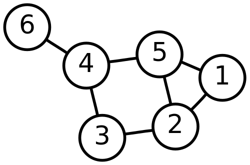
There are multiple ways to implement graphs. One could take an object oriented approach, where node objects have pointers to their children. Another more common method is to use neighbor-lists or matrices, where each entry represents a connection in the graph.
Neighbor Lists
Given the graph G with nodes
To clarify,
Neighbor Matrices
For dense graphs, graphs with relatively many edges, neighbor-matrices may prove more useful for representing edges. For a graph with
    0 1 2 3 4 5
  -------------
0 | 0 1 0 0 0 1
1 | 0 0 1 1 0 1
2 | 1 1 0 1 0 0
3 | 0 0 1 0 1 0
4 | 0 0 0 0 0 1
5 | 1 0 1 0 1 0
This matrix represents a graph
Traversal
Now that we have a representation for graphs it is possible to traverse the nodes through the nodes. The two most common methods of traversal are Breadth First Search (BFS) and Depth First Search (DFS).
Breadth First Search (BFS)
Breadth first search is a graph traversal algorithm that as it examines a node, it adds all of that node's children to the queue. More precisely:
- The input is a graph and a starting node. The algorithm uses a queue to establish in which order it visits each node. The first node added to the queue is the starting node.
- As long as there exists elements in the queue, the algorithm removes (dequeues) the first element from the queue, mark the node as visited, then enqueue it's children.
BFS can mark each node with a distance value, which indicates how many edges away it is from the starting node. Also, if you are searching for an element using BFS, the search can be terminated when the node you are searching for is found and dequeued.
Runtime:
Depth First Search (DFS)
DFS is similar to BFS, but uses a stack instead of a queue. Since a stack is LIFO, each child node is pushed onto the stack until a leaf node is reached. The node on the top of the stack is then popped, handled and discarded before moving to the underlying node. More precisely:
- The input is a graph and a starting node. The algorithm uses a stack to establish in which order it visits each node. The first node added to the stack is the start node.
- The algorithm pushes child nodes to the stack until a leaf node is reached. The topmost node on the stack is then handled, and this repeats until a node has children.
DFS cannot find the distances between nodes in a graph, but can record how many nodes it visited before adding the node in question onto the stack, as well as when it removed said node from the stack. This is called start and stop times, which can prove useful for topological sorting.
Runtime:
Traversing order
In-order traversal, pre-order traversal, and post-order traversal all traverse nodes in the same order, the difference is when each node is handled (sometimes called visited or colored). When traversing a tree, these traversal methods work in the following way:
- In a pre-order traversal, nodes are handled before visiting any subtrees.
- In an in-order traversal, nodes are handled after visiting the left subtree.
- In a post-order traversal, nodes are handled after visiting the both subtree.
| Traversal method | Visualization | Result |
| Pre-order |  |
F, B, A, D, C, E, G, I, H |
| In-order |  |
A, B, C, D, E, F, G, H, I |
| Post-order |  |
A, C, E, D, B, H, I, G, F |
Minimal Spanning Trees
A minimal spanning tree is a tree that is connects to all nodes exactly once, and has the lowest possible cumulative edge weight.
Kruskal
Kruskal's algorithm creates a tree by finding the smallest edges in the graph one by one, and creating a forest of trees. These trees are gradually merged together into one tree which becomes the minimal spanning tree. First the edge with the smallest weight is found and this edge is made into a tree. Then the algorithm looks for the second smallest edge weight and connects these two nodes. If these were two free nodes they are connected as a new tree; if one of them are connected to an existing tree, the second node is attached to that tree; and if both are in separate trees these two trees are merged; if both are in the same tree then the edge is ignored. This method continues until we have one complete tree with all nodes.
| Best Case | Average Case | Worst Case |
Prim
Prim's algorithm creates a tree by starting in an arbitrary node and then adding the edge (and connecting node) with the smallest weight to tree. With now two nodes connected, the edge with the lowest weight that connects to either of the two nodes is added. This continues until all of the nodes have become a part of the tree. Runtime depends on the underlying data structure, however the curriculum uses a binary heap.
| Best Case | Average Case | Worst Case |
Shortest Path
Finding the shortest path between two nodes is a common problem. It can be applied to for instance finding the the best GPS route.
In general, shortest path problems are divided into subproblems where we look at the shortest stretches between nodes.
Typical issues of concern when selecting an algorithm is:
-
Is the graph directed or undirected (ordinary)?
-
Are there negative edges?
-
Do cycles exist in the directed graph? If the cycle is positive, there will always be a shorter path that does not include the cycle.
-
Are negative cycles created? In this case, finding a shortest non-simple path is impossible.
One-to-All
One-to-all means finding the distance to all notes from a single starting node.
Relax
Relax is a function which shortens the estimated distance to a node
An important property of relax is that if
Dijkstra's algorithm
Dijkstra's algorithm only works if all edges are non-negative.
| Best Case | Average Case | Worst Case |
If one or more negative cycles exist, this algorithm will not terminate as normal. It is possible to add an alternative stopping method, however the result may be wrong.
Dijkstra is most effective when used in a heap. Implementation in other structures can cost higher runtimes and are not in the curriculum.
How it works:
- Initialize distances; Set the starting node to
$0$ and all others to$\inf$ . - Initialize visited; Set the startnode to visited, and all other to not visited.
- Look at all neighbors; Calculate and update distances.
- Go to a node which hasn't been visited, and with the lowest distance value from start. Mark it as visited.
- Repeat steps
$3$ -$5$ until all nodes have been visited or an specific end node is visited.
In python:
def dijkstra(G,start): #G er grafen, start er startnoden
    pq = PriorityQueue() # initialiserer en heap
    start.setDistance(0) # Initialiserer startnodens avstand
    pq.buildHeap([(node.getDistance(),node) for node in G]) # Lager en heap med alle nodene
    while not pq.isEmpty():
        currentVert = pq.delMin()    # velger greedy den med kortest avstand
        for nextVert in currentVert.getConnections():
            newDist = currentVert.getDistance() + currentVert.getWeight(nextVert) #kalkulerer nye avstander
            if newDist < nextVert.getDistance():
                nextVert.setDistance( newDist ) # oppdaterer avstandene
                nextVert.setPred(currentVert) # Oppdaterer foreldrene til den med kortest avstand
                pq.decreaseKey(nextVert,newDist) # lager heapen på nytt så de laveste kommer først.
Bellman-Ford
Unlike Dijkstra, Bellman-Ford works also with negative edges.
| Best Case | Average Case | Worst Case |
Bellman-Ford is defined recursively. In contrast to Dijkstra, Bellman-Ford relaxes all edges multiple times. This helps discover any potential negative cycles. All edges are relaxed
How it works:
- Initialize the algorithm by setting the distance from the startnode to 0, and all others to +inf.
- Compare all distances, and update each node with the new distance.
- Run one more iteration to check for negative cycles.
In python:
def bellman_ford(G, s) # G er grafen, med noder og kantvekter. s er startnoden.
    distance = {}
    parent = {}
    for node in G: # Initialiserer startverdier
        distance[node] = float('Inf')
        parent[node] = None
    distance[s]=0 # initialiserer startnoden

    # relax
    for (len(G)-1):
        for u in G:    # fra node u
            for v in G[u]:    # til naboene
                if distance[v] > distance[u] + G[u][v]: # Sjekker om avstanden er mindre
                    distance[v] = distance[u] + G[u][v]    # hvis ja, oppdaterer avstanden
                    parent[v]=u    # og oppdaterer parent

    # sjekk negative sykler
    for u in G:
        for v in G[u]:
            if distance[v] > distance[u] + G[u][v]:
                return False
DAG shortest path
It is possible to topologically sort a DAG (Directed Acyclic Graph) to find the correct order in which to relax each edge to find the shortest one-to-all path.
Psuedocode from Cormen:
1 DAG-SHORTEST-PATHS(G, w, s)
2    for each vertex v in G.V
3        v.d = inf  # Distance
4        v.p = null # Parent
5    s.d = 0
6    for each vertex u in G.v, where G.v is topologically sorted
7        for each adjacent vertex v to u
8            if v.d > u.d + w(u, v) # Relax
9                v.d = u.d + w(u, v)
10               v.p = u
| Best Case | Average Case | Worst Case |
All to All
Johnson's algorithm
Johnson's algorithm combines Dijkstra and Bellman-Ford such that it finds an all-to-all distance matrix for graphs. It allows graphs with negative-weight edges, but not negative-weight cycles. It works best with graphs with few edges.
How it works:
Let
The following is pseudocode of Johnson's algorithm.
1  G_s = construct_G_with_start_node_s()
2  Bellman_Ford(G_s, s)
3  for node in G.nodes
4      h(node) = G_s.node.distance #distance s to node
5  for edge in G.edges
6      edge.weight = edge.weight + h(edge.parent) - h(edge.child)
7  D = matrix(n, n) #some n*n matrix
8  for node_I in G.nodes
9      Dijkstra(G, node_I) #uses dijkstra to find distances from node "node_I" with updated edge.weights in G
10     for node_J in G.nodes
11         D[I, J] = node_J.distance + h(edge.child) - h(edge.parent) #add all distances starting in node I to the matrix
| Best Case | Average Case | Worst Case |
Floyd-Warshall
FW works even if there are negative edges, but no negative cycles. The nodes must be stored as a neigbor matrix not a list.
Psuedocode from wikipedia:
1 let dist be a |V| × |V| array of minimum distances initialized to ∞ (infinity)
2 for each vertex v
3    dist[v][v] ← 0
4 for each edge (u,v)
5    dist[u][v] ← w(u,v)  // the weight of the edge (u,v)
6 for k from 1 to |V|
7    for i from 1 to |V|
8       for j from 1 to |V|
9          if dist[i][j] > dist[i][k] + dist[k][j]
10             dist[i][j] ← dist[i][k] + dist[k][j]
11         end if
In Python:
def FloydWarshall(W):
    n = len(W)
    D = W
    PI = [[0 for i in range(n)] for j in range(n)]
    for i in range(n):
        for j in range(n):
            if(i==j or W[i][j] == float('inf')):
                PI[i][j] = None
            else:
                PI[i][j] = i

    for k in range(n):
        for i in range(n):
            for j in range(n):
                if D[i][j] > D[i][k] + D[k][j]:
                    D[i][j] = D[i][k] + D[k][j]
                    PI[i][j] = PI[k][j]
    return (D,PI)
| Best Case | Average Case | Worst Case | |
| linear arr | |||
| binary he | |||
| binary he |
The Algorithm creates matrix
Max Flow
Flow can be visualized by forexample a pipe system to deliver water to a city, or as a network with differing capacity on the various cables. Max fow is the maxium net capacity that actually flows through the network. There may exist some critical pipes (edges) with very low capacity, bottlenecking the entire network no matter the size of the other pipes. Max flow is achieved when there exists no more augumenting paths.
Flow Network
A flow network is a directed graf where all the edges have a non-negative capacity. Additionally, it is required that if there exists an edge between u and v, there exists no edge in the opposite direction from v to u. A flow network has a source, s, and a sink, t. The source can be seen as the starting node and the sink as the end node. The graph is not divided so for all v there exists a route s ~v~t. All nodes except from s have atleast one inbound edge. All nodes except the source and the sink have a net flow of 0 (all inbound flow = all outbound flow).
A flow network can have several sources and sinks. To eliminate this problem, a super source and super sink are created and linked up to all respective sources and sinks with edges that have infinite capactiy. This new network with only one source and sink is much easier to solve.
Residual Network
The residual network is the capacity left over:
To keep an eye on the residual network is useful. If we send 1000 liters of water from u to v, and 300 liters from v to u, it is enough as sending 700 from u to v to achieve the same result.
Augumenting Path
An augumenting path is a path from the source to the sink that increases the total flow in the network. It can be found by looking at the residual netowrk.
Minimal cut
A cut in a flow network divides the graph in two, S and T. It is useful to look at the flow through this cut:
Of all possible cuts, we want to see the cut with the smallest flow, as this is the bottleneck of the network. Proof exists that show that finding the minimal cut simultaneously gives us the maximum flow through the network.
Ford-Fulkersons method
Given flow f, in each iteration of Ford-Fulkerson we find an augumenting path p, and use p to modify f.
| Best Case | Average Case | Worst Case |
Edmonds-Karp
Edmonds-Karp is Ford-Fulkerson's method where BFS is the traversal method. This ensures a runtime of
Whole Number Theorem
If all capacities in the flow network are whole numbers, then Ford-Fulkerson's method will find a max flow with a whole number value, and the flow between all neighbor nodes will have whole number values.
Dynamic Programming
Dynamic programming divides up problems into smaller subproblems, just like divide-and-conquer. DP can be used when there is both optimal substructure and where subproblems overlap.
It is often possible to use divide-and-conquer on these types of problems, but often a lot of redundant work is done, I.E. the same subproblem is solved several times. DP only needs to solve a subproblem once, and then uses the result each time it is needed.
DP is usually used for optimization problems, but as there can be several optimal solutions it is one of many optimal solution.
- Characterize the structure of the optimal solution.
- Recursively define the value of an optimal solution.
- Compute the value of an optimal solution, typically in a bottom-up fashion.
- Construct an optimal solution from computed information.
Longest common substring
Is solved by DP from the bottom up, by looking at the last element
Rod-cutting
Given a rod with length
We can cut up a rod on length
Greedy Algorithms
Some times a DP is a bit overkill. Greedy algorithms choose the solution that seems the best righ tthen and there, and moves on. This does not always leed to the best solution, but for many problems this works fine. Minimal spanning trees is an example of a greedy method. Greedy algorithms solve the problem if it has the following attributes:
-
$Greedy-choice\ property$ We can make a choice that seems optimal at the time and solve the subproblems that occur later. The greedy choices can not be dependent on future choices nor all existing solutions. It simply iteratively takes greedy choices and reduces the given problem to a smaller one. -
$Optimal\ substructure$ Optimal solitions to a problem incorporate optimal solutions to related subproblems, which we may solve independently.
Planning activities
Choose as many non-overlapping activities as possible. Assume that they are sorted by ending time and use a greedy algorithm to select them.
Huffman's algorithm
Huffman's algorithm is a greedy algorithm with the intent to minimize saving space to a known sequence of symbols. Each symbol can be represented by a binary code. The given code is dependent on the frequency the symbol, where the more frequent terms get the shorter bits. Depending on term distribution, this reduces the space required by 20-90%.
Huffman is performed by always summing the two nodes with the smallest frequency values, and then using the num of these as the value of a new node. By branching left with
Runtime:
| Best case | Average case | Worst case |
One version of Huffmann coding can look like this:

Multithreading
The basics of Multithreading
Concurrency keywords
- Spawn - used to start a parallel thread, allowing tha parent thread to continue with the next line while the child thread runs its subproblem
- Sync - A procedure cannot safely use the values returned by its spawned children until after it executes a sync statement. This keyword indicates that the program must wait until both threads are finished allowing for the correct variables to syncronize
- Serializaion - the serial algorithm that results from deleting the multithreaded keywords: spawn, sync, and parallel.
- Nested parallelism - occurs when the keyword spawn precedes a procedure call. A child thread is spawned to solve the subproblem which in turn runs their own spawn subproblems, potentially creating a vast tree of subcomputations, all excecuting in parallel.
- Logical parallelism - concurrency keywords express logical parallelsism, indicating which parts of the computation may procedd in parallel. At runtime it is upt o a scheduler to determine which subcomputations actually run concurrently.
Performance Measures
Two metrics, work and span.
Work - The work of a multithreaded computation is the total time to execute the entire computatin on one processor. It is the sum of the times taken by each strand.
Span - The span is the longest time to execute the strands along any path of the DAG. Again for a DAG in which each strand takes unit time, the span equals the number of vertices on a longest or critical path in the DAG. Given that time to calculate is denoted as
- Rewriting the work law we get
$T_1/T_P \leq P$ , stating that the speedup on P processors can at most be P. - If
$T_1/T_P = \theta(P)$ implies linear speed up -
If
$T_1/T_P = P$ implies perfect linear speed up -
The ratio
$T_1/T_\infty$ of the work to the span gives the parallelism of the multithreaded computation.
Problem Complexity
P, NP, NPC
The question connected to whether
 We know that
| P | Polynomial time | |
| NP | Nondeterministic polynomial time | |
| NPC | Nondeterministic polynomial time complete | |
| NPH | Nondeterministic polynomial time hard |
That a problem is P, implies it is solvable in polynomial time. An NP-problem is a problem that we can prove is true (verifiable), at polynomial time. If it is possible to falsify the solution in polynomial time, the problem is a part of the co-NP-class. NP-Hard (NPH) problems cannot be solved in polynomial time. It is said that this class of problems are atleast as difficult as the most difficult problem in the NP-class. In other terms, they are problems which can be reduced from NP-problems in polynomial time, but not necessarily allows themselves to be verified in polynomial time with a given solution. NP-hard problems that allow themselves to be verified in polynomial time are called NP-complete.
Reducibility-relation
To understand the proof technique used to prove a problem is NPC, a few definitions need to be in place. One of these is the reducibility-relation
Cormen et al., exemplifies that the linear equation
Some known NPC problems
Some common examples of NPC problems include:
- Circuit-SAT
- SAT
- 3-CNF-SAT
- Clique-problemet
- Vertex-Cover
- Hamilton-Cycle
- Travelling Salesman (TSP)
- Subset-Sum
But how can we prove a poblem is NPC?
Cormen et al. divides this into two parts:
- Prove that the problem belongs to the NP-class. Use a certification to prove that the solution is verified in polynomial time.
- Prove the problem is NP-hard. This is done through polynimial time reduction.
Given
This connection is illustrated in the figure below:

Given that you are trying to prove that TSP is an NPC-problem:
- Prove that TSP
$\in$ NP. The certification you use can be a sequence of n nodes that you shall visit on your trip. If the sequence just consists of unique nodes (we do not visit the same city more than oce) then we can sum up the costs and verify the total cost is less than a given number k. - Prove that TSP is NP-hard. If you have understood what the different problems described above, then you will recognize that TSP is a Hamilton Cycle-problem (given an undireted graph G, there exists a cucle that contains all the nodes only once, and where the starting node = the end node). We know that TSP is atleast as difficult to solve as a the Ham-cycle problem (as Ham-cycle is a subproblem of TSP). Given that we already have proved that the Ham-cycle problem is NP-hard, we can show with polynomial time reduction that TSP is also NP-hard (since we reduce Ham-cycle to TSP in polynimial time, then TSP is NP-H)
As most people now believe that
Runtimes for curriculum algorithms
Sorting and selection
$n$ is the number of elements that are being handled.$k$ is the highest value possible.$d$ is the max munber of digits an element can have.
| Algorithm | Best case | Average case | Worst case | Space Complexity Worst Case | Stable |
| Merge sort | Yes | ||||
| Quick sort | No | ||||
| Heap sort | No | ||||
| Bubble sort | Yes | ||||
| Insertion sort | Yes | ||||
| Selection sort | No | ||||
| Bucket sort | Yes | ||||
| Counting sort | Yes | ||||
| Radix sort | Yes* | ||||
| Select | NA | NA | |||
| Randomized select | NA | NA |
- Radix sort need require a stable sub-sort for itself be stable
Heap-operations
| Operations | Runtime |
| Insert | |
| Delete | |
| Build | |
| Max-heaplify | |
| Increase-key | |
| Maximum |
Graph-operations
| Algorithm | Best case | Average case | Worst case |
| Topological sort | |||
| Depth-first-search | |||
| Breadth-first-search | |||
| Prim's | |||
| Kruskal's | |||
| Bellmann-Ford's | |||
| Dijkstra's | |||
| Floyd-Warshall's | |||
| DAG-shortest-path |