TMA4115: Calculus 3
Complex numbers
"A complex number is a number that can be expressed in the form
Modulus
Essentially the length of the vector from the origin to
Argument
The line from the origin to (a, b) has an angle
Polar form
Given
Multiplication
Division
Complex form
Euler's formula:
Based on that formula, we can write a complex number
Roots
When finding the
First, write
Next comes the most important step: raise both sides to the power of
Note: If you try to insert
Complex functions
Second order linear differential equations
Linear, homogenous equations with constant coefficients
Distinct real roots
Complex roots
Repeated roots
Inhomogeneous equations
The inhomogenous linear equation
In order to find
- Undetermined coefficients
- Variation of parameters
Harmonic oscillator
Step 1:
Solve the homogenous equation by solving the characteristic equation
if
if
if
Step 2:
Compute
General solution:
Vectors
A vector in this subject is always thought of as a column vector, and is written as such:
Normalization of vectors
When we normalize a vector we are making the length of the vector
Matrices
Terminology
For example, when a text says "Suppose a 4 x 7 matrix A (...)", that means that m = 4, n = 7. Can't remember the order? Rule of thumb: Just remember the word "man" and that m comes before n. m is the height of the matrix, and n is the width of the matrix.
Linear transformations
A matrix can be regarded as a transformation that transforms a vector. For example, a transformation
Onto and one-to-one
Let
$T$ is onto if and only if the columns of$A$ span$\mathbb{R}^m$ . In other words,$Ax = b$ has a solution for each$b$ in$\mathbb{R}^m$ .$T$ is one-to-one if$A$ is invertible, i.e. the columns of$A$ are linearly independent.
Inverse of a matrix
The inverse of a matrix
For example, consider the following matrix
To find the inverse of this matrix, one takes the following matrix augmented by the identity, and row reduces it as a 3 by 6 matrix:
By performing row operations, one can check that the reduced row echelon form of the this augmented matrix is:
By this point we can see that B is the inverse of A.
A matrix is invertible if, and only if, its determinant is nonzero.
LU factorization
With this technique, you can write
First, write down the augmented matrix:
Why LU factorization?
Because when
Determinants
The determinant of a 2x2 matrix is simple to compute. Here's an example:
Calculating the determinant of a larger matrix is harder. Look up "cofactor expansion" in your textbook or on the internet. Moreover, here are some useful theorems related to determinants:
-
If
$A$ is a triangular matrix, then$det\: A$ is the product of the entries on the main diagonal of$A$ . -
Adding one row of
$A$ to another row of$A$ will not change$det\: A$ . -
A square matrix
$A$ is invertible if and only if$det\: A \neq 0$ .
Eigenvalues and eigenvectors
Eigenvalues and eigenvectors apply to square matrices.
Eigenvalue
Definition
An eigenvalue is a value that satisfies this equation:
To find the eigenvalues you evaluate the definition.
This is where
An example of finding the eigenvalues of a matrix
Given the matrix:
The roots of this polynomial are
Eigenvectors
After we have found the eigenvalues, we can find the eigenvector.
The eigenvectors are the vectors that satisfy the equation:
2D rotation matrix
Given that
The eigenvalues of
Then
Column Space and Null Space of a Matrix
The column space of a matrix A is the set Col A of all linear combinations of A. The vector
If
The rank of a matrix
The null space of a matrix A is the set Nul A of all solutions of the homogeneous equation
Basis
Col A: The pivot columns of A form a basis for the column space of A. Be careful to use the pivot columns of A itself for the basis of Col A, not the columns of an echolon form B.
Row A: The row space is not affected by elementary row operations. Therefore, the non-zero rows of the matrix in echelon form are a basis for the row space.
Orthogonality
A set of vectors is orthogonal if the vectors in the set are orthogonal (perpendicular) to each other. Two vectors
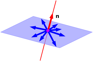
Orthogonal complement
The set of all vectors
Orthonormal set
An orthonormal set is orthogonal, but has one extra requirement: Every vector has length equal to 1.
If you construct a matrix
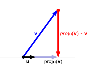
Projection
The Gram-Schmidt process
Let's say that you have a set of linearly independent vectors. The Gram-Schmidt process can orthogonalize these vectors.
Example:
QR factorization
If
You can use the Gram-Schmidt process for finding
Symmetric matrices
A symmetric matrix is a square matrix
For any symmetric matrix
If
Useful links
Recap lecture (Norwegian)
Course videos (Norwegian)
Second order differential equations on Khan Academy
Linear algebra on Khan Academy
Official website with homework assignments, old exams etc.
Differential Equations explained